The right decision is to refuse to take the jab. The consequences of that decision will be less in the long run, for members of the U.S. military, for all children, for women who hope to bear children, for employees and anyone else who is being forced to take the jab. Your body and the bodies of your children and grandchildren do not belong to the government. Advocate for yourself and your family.
Posted August 18, 2021 by budbromley. Revised January 18, 2024. Thanks to Brendan Godwin for editorial suggestions.
In physical chemistry, Henry’s Law is one of the gas laws. It defines the solubility of a gas within a liquid which is in contact with the same gas above the surface of the liquid. It was formulated in the early 19th century by the William Henry, M.D., and Englishman who practiced chemistry, owned a family business for carbonated beverages, and described his extensive experiments with gases and liquids in a series of books reviewed by John Dalton (of the gas laws and atomic weights) and published by the Royal Society of London. In the 21st century, Henry’s Law is the foundation science for multi-billion per year industries, for example the multi-billion dollar per year scientific instruments business of gas chromatography. Henry’s Law also explains the theory of human-caused global warming /climate change is not even plausible science and should be shunned by knowledgeable people.
Henry’s Law is specifically limited to a physical phase state equilibrium of a specified gas which is in continuous contact with a liquid, and as far as known applies to all solute gases and solvent liquids, for example CO2 gas in the atmosphere which is in contact with ocean water. In that phase state equilibrium Henry’s Law defines the concentration of the gas dissolved in the liquid surface divided by the concentration of that same gas in space above the liquid surface. Typically, and specifically for the gold standard CO2 measurements, the units are moles of CO2 per mole of dry air, or per mole of liquid. This is not a volumetric measurement. This ratio or coefficient is the dimensionless version of the Henry’s Law constant, one of several useful derivations for different purposes. This dimensionless version is convenient since the units are the same as used by NOAA-Scripps Global Monitoring Labs (GML), which measures net atmospheric CO2 as micromoles CO2 per mole of dried air. The ratio of these two molar concentrations (e.g., moles of CO2 gas in liquid surface per mole of CO2 gas in dry air) is the Henry’s Law constant or coefficient; it is sometimes known as an Arrhenius constant because it varies with temperature. The molar concentration of CO2 gas in the liquid phase increases as temperature of the liquid surface decreases. The Henry’s Law constant for CO2 and seawater increases significantly as temperature of the sea water surface declines.
Thus, the Henry’s Law phase-state equilibrium constant is dynamically changing as the temperature of the liquid changes, apparently a much less familiar concept to scientists. This physical phenomenon enables temperature programming in gas chromatography and efficient, precise and accurate separation of components in mixtures of chemicals, a multi-billion dollar per year industry.
Henry’s law only applies to low concentrations of a gas in the mixed gas phase (typically air) and low concentrations of the solute gas in the liquid solvent phase. Henry’s Law does not apply to the reaction products of a gas which has reacted with the liquid.
CO2 gas in the atmosphere and in ocean surface satisfies these conditions.
Henry’s Law does not apply to the series of carbonate chemistry reactions occurring in ocean water after the CO2 gas has reacted with water ions, and thereby hydrated and disassociated into ions. Henry’s Law and its partition ratio only apply to the unreacted, non-ionized CO2 gas in the water and in the air above the water. Most of theCO2 gasabsorbed in water reacts with water ions or other ions in water to produce either carbonate (as carbonic acid) or as bicarbonate ions.
Henry’s Law is dominantly dependent on (i.e., a function of) the temperature at the interface surface between the gas and the liquid. The density of the surface thin layer matrix is decreased by increasing temperature of the surface, and the activity, molecular and ionic vibrations, is increased in the surface thin layer matrix by temperature increase, and these phenomena result in an increased emission rate of the solute gas from the liquid surface. The reverse occurs when the liquid surface is cooled, resulting in increased absorption and solubility of the gas in the liquid surface. These phenomena hold for all gases and liquids.
Rearranging Henry’s Law as d(ln(kH))/d(1/T) defines the temperature dependence parameter in Henry’s Law partition co-efficient, where kH is the Henry’s Law constant and T is temperature in Kelvin. Henry’s Law is explained on the website of the U.S. National Institutes of Standards and Technology. https://webbook.nist.gov/cgi/cbook.cgi?ID=C124389&Units=SI&Mask=10#Solubility
“The chemistry of carbon dioxide is quite complex, but it boils down to reactions as in Eq. (I). In the first step, CO2 of the atmosphere dissolves into the ocean CO2(g)⇌CO2(aq). (I)
In water the CO2 molecules combine with water molecules to form H2CO3 , and this reaction can be written as CO2(aq)+H2O(l )⇌H2CO3(aq). (II)
Here the ratio of the two concentrations of Eq. (I) is given by Henry’s Constant, that depends on the temperature (see Table 6-7 of Lide and Frederikse (1974)), 𝐾h(𝑇)= [CO2(g)] / [CO2(aq)]. (3)” (Stallinga, P. (2018). Carbon Dioxide and Ocean Acidification. European Scientific Journal, ESJ, 14(18), 476. https://doi.org/10.19044/esj.2018.v14n18p476 )
Since the concentration of net global CO2 gas concentration is routinely measured, Henry’s Law can be used to calculate the concentration of aqueous CO2 gas in ocean surface water. This is the best method to calculate CO2 gas concentration in seawater since the hydration reaction and the first two carbonate reactions are very fast and reversible by changes in temperature, agitation, pH, salinity, and partial pressure.
Theoretically, this concentration of aqueous CO2 gas then can be used to roughly calculate the concentration of the carbonates in the series of acid-base reactions in ocean water which occur after the hydration reaction, but there are many different equilibrium constants involved, and ocean and atmosphere are very dynamic media. These reactions subsequent to ionization of CO2 gas in water are not described by Henry’s Law constant.
Using average global temperature or average sea surface temperature (SST) in Henry’s law calculations results in errors unless that average SST is weighted by surface area at the temperature used for the Henry’s constant. However, I have not found this information in the scientific literature except with regard to Fick’s Law as follows. Adolph Fick’s 1st Law describes net flux of gases through surfaces, membranes and tissues, such as alveolar lung tissue or leaves. Fick’s Law will be described in detail in another post.
Use of a global average temperature results in unexplained errors and uncertainties in the gas concentrations. CO2 is highly and rapidly soluble in water and its solubility increases as water temperature declines, that is, CO2 gas solubility in water is inversely proportional to temperature of the water. Thus Henry’s Law constants are presented in text books with a reference temperature.
For example, global average ocean temperature is about 17 C, which subject to the Henry’s coefficient defines ocean net CO2 flux as a net absorbing sink for CO2. This leads to the question: how can global average CO2 concentration be increasing if average ocean temperature is 17 C? But the average temperature of the tropical ocean surface is about 26 C year-round, which implies net CO2 flux from tropical ocean surface is a net emitting CO2 gas source year-round. Thus, the Henry’s Law constant for CO2 and ocean water depends on the relative surface area per SST. In other words, when the sea surface area increases for SST 26 C relative to the surface area for 17 C, then net CO2 emission flux increases; units would be analogous to moles of CO2 gas emitted per square kilometer of sea surface per year.
Henry’s Law constants are intensive properties of matter which describe the proportion of a gas in a liquid at a given temperature as a ratio with the same gas in the space above and in contact with the liquid. The ratio is the intensive property.
A few examples of common errors in the climatology literature are provided below.
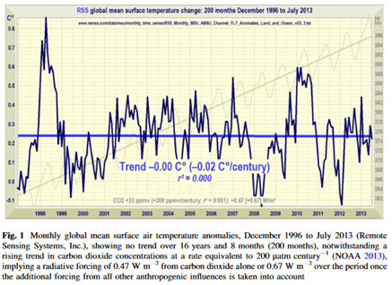
In the following graph, the carefully measured net global CO2 trend or net flux (measured at Mauna Loa, the gray sawtooth line and its mean trend, the thin gray line) is shown versus the RSS satellite-measured global mean surface temperature (the jagged bold black line and its blue mean trend line.) The two trends (CO2 and temperature) are strongly diverging with respect to time which falsifies anthropogenic global warming (AGW) theory; the calculus theorem is the subject of another paper. Global mean surface temperature is essentially trendless in recent decades, while net atmospheric CO2 (i.e. all emissions minus all sinks) in the same years has been increasing about 2.5 ppm per year but the human contribution is only a fraction of that 2.5 ppm; how is it rational to claim that human CO2 dominantly from fossil fuels is the cause of global warming/climate change?
An intensive property of matter depends only on the type of matter and not on the amount of matter and nor its source and may vary from place to place within the system at any moment. The average temperature of the earth and the average temperature of earth’s troposphere, average global SST, and surface air temperatures provide no useful information regarding CO2 net flux nor Henry’s Law constants and result in errors in calculating net atmospheric CO2 concentration and net flux. For example, using Henry’s Law and average sea surface temperature of 17 C calculates an average global CO2 concentration of about 312 ppm, which would obviously be a large error based on Mauna-Loa-observed net global average CO2 concentration of about 417 ppm.
Henry’s Law and its partition ratio (aka constant or co-efficient) for CO2 and water apply only to this equilibrium reaction: CO2(g)⇌CO2(aq)
where CO2(g) is the CO2 gas in the gas phase headspace above the liquid surface
and CO2(aq) is the CO2 gas dissolved in the liquid phase.
In this initial hydration reaction, CO2(g) has not disassociated. It is a gas dissolved in liquid water.
Henry’s Law does not apply to the reaction products subsequent to the hydration reaction of CO2(aq) nor to the subsequent reactions of those products. The stoichiometric ratio of the two concentrations of this first phase state reaction [CO2(g)]⇌[CO2(aq)] is given by the Henry’s co-efficient which depends on temperature (see for example Table 6-7 of Lide and Frederikse (1974), or the Handbook of Chemistry and Physics found in almost all chemistry labs.)
Henry’s Law determines the exchange rate of CO2(g) between the estimated 1000 gigatonnes CO2(g) dissolved in ocean surface and the estimated 700 gigatonnes of CO2(g) in the atmosphere; the exchange rate is estimated as two 90 gigatonnes CO2 per year fluxes moving continuously in opposite directions, into air and also into ocean surface continuously. This is illustrated in Figure 17.11. For comparison, humans are estimated to emit into air about 8 gigatonnes of CO2 per year, which is immediately, chaotically mixed with the two 90 gigatonne fluxes, one estimated flux out of ocean, land and biosphere and one estimated flux into ocean, land and biosphere. That is, these two fluxes are each about 10 times larger than annual human CO2 emissions. Fick’s 1st Law describes the net difference between these two vector directional fluxes. The Keeling Curve, which is the generally accepted defacto gold standard produced diligently by the NOAA-Scripps Global Monitoring Lab at Mauna Loa (MLO), is the time derivative of Fick’s 1st Law for CO2 net flux into and out of earth’s environment.
In most climatology literature, aqueous CO2 gas is bundled together and summed with carbonic acid, bicarbonate and carbonate anions in the several initial carbonate chemistry reactions and is usually quantified within the total millimol/kg-of-solution dissolved inorganic carbon (DIC). This practice has apparently led to wide-spread misunderstanding of Henry’s Law. As previously stated, Henry’s Law does not apply to the products of gas solutes which have reacted with liquid solvents. Each of these carbon moieties on the reactants side and the products side vary based on multiple factors, mainly temperature of the ocean surface, salinity, alkalinity, and CO2 gas concentration (or partial pressure) in air immediately above the ocean surface, and CO2 gas concentration in the ocean surface. Consequently, the important Henry’s phase-state equilibrium has been ignored or confused in climate literature resulting in significant, unexplained errors in the literature. For example, DIC is directly proportional to CO2(g) ppm in air, but DIC is inversely proportional to ocean surface temperature. If CO2(g) is constant at 400 ppm, then DIC is inversely proportional to ocean temperature while pH is directly proportional to temperature. Clearly it is mistaken to bundle these co-dependent offsetting chemical entities into a single one-dimensional hypothetical reactant. http://www.molecularmodels.eu/Ocean-CO2.pdf
“The analysis of dissolved CO2 in water is an important basis for the assessment of the role of surface waters in the global carbon cycle (Raymond et al., 2013). Indirect methods like calculating CO2 from other parameters like alkalinity and pH (Lewis and Wallace, 1998; Robbins et al., 2010) are affected by considerable random and systematic errors (Golub et al., 2017) caused for example by dissolved organic carbon, which may result in significant overestimation of the CO2 partial pressure (pCO2) (Abril et al., 2015), or by pH measurement errors (Liu et al., 2020). Thus, direct measurement of CO2 is highly recommended, particularly in soft waters.”Koschorreck, M., Prairie, Y. T., Kim, J., and Marcé, R.: Technical note: CO2 is not like CH4 – limits of and corrections to the headspace method to analyse pCO2 in fresh water, Biogeosciences, 18, 1619–1627, https://doi.org/10.5194/bg-18-1619-2021, 2021.
“Measurements of the atmospheric CO2 concentration indicate that it has been increasing at a rate about 50% of that which is expected from all industrial CO2 emissions. The oceans have been considered to be a major sink for CO2. Hence the improved knowledge of the net transport flux across the air–sea interface is important for understanding the fate of this important greenhouse gas emitted into the earth’s atmosphere (1–5).” … “Sources of Errors. The flux estimates are subject to errors from the following five independent sources: (i) the gas transfer coefficients, (ii) the wind speed variability, (iii) the normalization of observations to the reference year of 1990, (iv) the interpolation of limited observations, and (v) skin temperature effect. “The estimated flux values, which range from 0.60 to 1.34 Gt-Czyr21, depend on the choice of sea–air CO2 gas transfer formulations. Hence the error is of a systematic nature and may be reduced if the gas transfer coefficient is better understood in the future.” Taro Takahashi et.al. Global air-sea flux of CO2: An estimate based on measurements of sea–air pCO2 difference. https://www.pnas.org/content/pnas/94/16/8292.full.pdf
While Henry’s law and temperature control the ratio of CO2 in air (i.e., CO2(g)) vs CO2 gas in ocean surface (i.e., CO2(aq)) in the physical phase-state reaction CO2(g)⇌CO2(aq), the enormous excess of aqueous CO2(g) in ocean is controlling the stoichiometry of the acid-base carbonate chemistry. The activities of carbonic acid, bicarbonate and other intermediate carbonate ions are constrained, being buffered (suppressed) by the 4 times excess of calcium ions and 1000 times excess of silicon ions with respect to carbonate ions in the well mixed upper ocean layer, resulting in highly buffered alkalinity in the ocean. Segalstad, Stumm and Morgan and others have pointed out that ocean water is an “infinite sink” for CO2. Ocean is infinitely buffered for CO2 gas; this means that in the hydration reaction CO2(g) + H2O(l) ⇌ H2CO3(aq), carbonic acid ( H2CO3), the weak acid created by hydrating CO2, can never make ocean acidic even if all know hydrocarbons on earth were burned and its CO2 emitted into the atmosphere. Weak carbonic acid is buffering ocean, preventing it from becoming too alkaline (Cohen & Happer, 2015).
The alkaline ocean and buffers for carbonate ions allow seawater to dissolve and react with huge amounts of aqueous CO2 gas, but that aqueous CO2 gas is only about 1% of the CO2 gas which was absorbed from air, the remaining ~99% is one of the products of reaction. Once hydrated into carbonic acid, the phase state reaction CO2(g)⇌CO2(aq) is unbalanced, which causes absorption of additional CO2 gas from atmosphere into the ocean surface. To calculate the true equilibrium value of CO2 gas in the air and aqueous CO2 in ocean surface at a given water temperature, all stoichiometry mass balances and kinetics of all of the carbonate chemical reactions must be simultaneously computed, accounting for the equilibrium constant of each reaction, and each of these reactions in turn depend on temperature, alkalinity, and salinity. These are complicated simultaneous differential equations.
In ocean water, CO2 gas molecules hydrate in seconds to form carbonic acid (H2CO3 ), but this does not mean the CO2(g)⇌CO2(aq) physical phase-state equilibrium can be ignored as usually done in climatology literature. Evidence of over 1000 gigatonnes of aqueous CO2 gas in ocean surface cannot be ignored. Also the hydration chemical reaction, i.e., aqueous CO2(g) + H2O(l) ⇌ H2CO3(aq), is more complicated than it is usually represented in climatology literature. Combining the CO2(g)⇌CO2(aq) physical phase-state reaction – which is controlled by Henry’s Law – with the CO2(g) + H2O(l) ⇌ H2CO3(aq) chemical hydration reaction and calling it simply HCO3* or H2CO3*, which are non-existing hypothetical entities, leads to stoichiometric errors in the various carbonate chemistry reactions as well as in the CO2(g)⇌CO2(aq) phase-state equilibrium reaction. The errors and uncertainty are often larger than the CO2 net emission flux that can be attributed to humans. For example in “Ocean pCO2 calculated from dissolved inorganic carbon, alkalinity, and equations for K1 and K2: validation based on laboratory measurements of CO2 in gas and seawater at equilibrium” by Timothy J LuekerAndrew G DicksonCharles D Keeling. https://www.sciencedirect.com/science/article/abs/pii/S0304420300000220. or https://doi.org/10.1016/S0304-4203(00)00022-0 The kinetics and stoichiometry of hydration and the chemistry and kinetics of CO2(g)⇌CO2(aq) phase-state reaction are omitted entirely.
The hydration equilibrium constant at 25°C for carbonic acid is [H2CO3]/[CO2] ≈ 1.2×10⁻³ in seawater. Hence, according to Alan L. Soli, Robert H. Byrne, the majority of the CO2 in sea water is not converted into one of the carbonate ions; it remains as aqueous CO2 gas molecules. Alan L. Soli, Robert H. Byrne, CO2 system hydration and dehydration kinetics and the equilibrium CO2/H2CO3 ratio in aqueous NaCl solution, Marine Chemistry, Volume 78, Issues 2–3, 2002, Pages 65-73, ISSN 0304-4203, https://doi.org/10.1016/S0304-4203(02)00010-5. https://www.sciencedirect.com/science/article/pii/S0304420302000105 Alan L. Soli, Robert H. Byrne, in this article and Cohen & Happer (2015) are contradictory on this point. This is merely to point out the contradiction in the literature.
Source: Stumm and Morgan. Aquatic Chemistry. Page 210.
This following short video explains the Henry’s Law equilibrium. Note also the University of California, Berkeley professor’s important comment about ammonia being “scrubbed” by water. In the same manner, CO2 is “scrubbed” from the air by water in ocean surface, soil, biosphere, bubbles, raindrops, animal lungs, etc. https://archive.org/details/ucberkeley_webcast_-ziliLAdom4
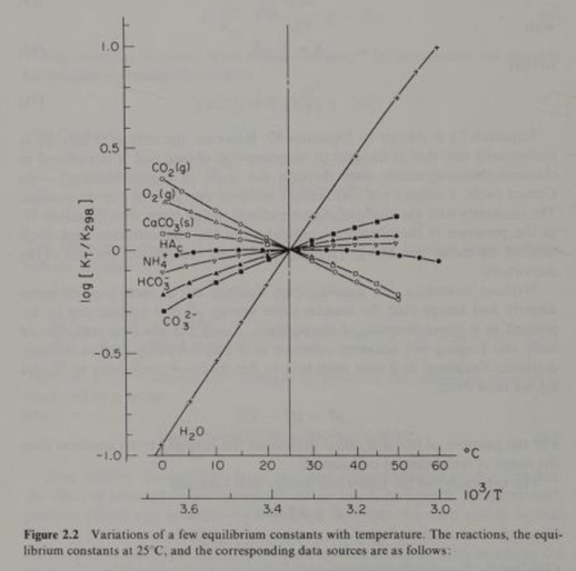
Figure 2.2 from Principles of Aquatic Chemistry, by Francois Morel. Hardcover Book, 446 pages. Description: An introductory text on aquatic chemistry, emphasizing a mathematical, quantitative approach to the field. Covers conservation of mass, thermodynamics and kinetics, chemical equilibrium calculations, acid-base, precipitation-dissolution, coordination, redox, and surface chemistry.
As mentioned, the Henry’s equilibrium “constant” or co-efficient for CO2(g) is not constant with respect to temperature. Also, the equilibrium “constants” for 3 other reactants and products in the initial carbonate chemistry series are not “constant” with respect to temperature. Figure 2.2 above from Morel illustrates significant variation in the equilibrium constants with respect to standard temperature (25 C). Clearly, bundling these offsetting, widely varying reactants and products together in a bundled hypothetical reaction will lead to errors.
“The Henry’s constant typically increases with temperature at low temperatures, reaches a maximum, and then decreases at higher temperatures. The temperature at which the maximum occurs depends on the specific solute-solvent pair.”…”It is important to recognize that the Henry’s “constant” is a strong, nonlinear function of temperature. For accurate design, it is preferable to have temperature-dependent data for Hi(T)… Additional pitfalls include failing to distinguish between the “solubility” and the “volatility” form of Henry’s law, failing to consider the implications of liquid-phase solute partitioning, and failing to be careful about units of measure, especially dimensionless units.”Harvey, A. and Smith, F. (2007), Avoid Common Pitfalls when using Henry’s Law, Chemical Engineering Progress, [online], https://tsapps.nist.gov/publication/get_pdf.cfm?pub_id=50449 (Accessed August 14, 2021).
Example papers of observed temperature-dependent CO2 emission or absorption or fugacity from ocean surface:
“Based on these observations, 72% of the increase in fCO2 sea [CO2 fugacity]in Cariaco Basin between 1996 and 2008 can be attributed to an increasing temperature trend of surface waters, making this the primary factor controlling fugacity at this location.” Astor, Y. M.; Lorenzoni, Laura; Thunell, R.; Varela, R.; Muller-Karger, Frank E.; Troccoli, L.; Taylor, G. T.; Scranton, M. I.; Tappa, E.; and Rueda, Digna, “Interannual Variability in Sea Surface Temperature and Fco2 Changes in the Cariaco Basin” (2013). Marine Science Faculty Publications. 1057. https://scholarcommons.usf.edu/msc_facpub/1057 . https://doi.org/10.1016/j.dsr2.2013.01.002
Note that the discussion and interpretations in the above paper attempt to support the theory of anthropogenic global warming (AGW). But, instead, the data in the paper support the case which is presented here. There are many papers like this in the scientific literature.
“Small changes in the largest marine carbon pool, the dissolved inorganic carbon pool, can have a profound impact on the carbon dioxide (CO2) flux between the ocean and the atmosphere, and the feedback of this flux to climate.” Irina I. Pipko, et.al. The spatial and interannual dynamics of the surface water carbonate system and air–sea CO2 fluxes in the outer shelf and slope of the Eurasian Arctic Ocean. Ocean Sci., 13, 997–1016, 2017 https://doi.org/10.5194/os-13-997-2017
“On the one hand, the hypothesis of Henry’s Law tells us that CO2 variations in the atmosphere are the result of temperature changes. We had already shown that for historical long-term data Henry’s Law is correct [ 12 23 ], as well as for periodic data of a specific meteorological station, De Bilt (Netherlands) [ 17 ].” … “Analyzing the contemporary data of Figure 3, we can conclude that Henry’s Law can readily explain this: every time warm water appears at the surface of the oceans, a huge amount of CO2 is released into the atmosphere (or less is absorbed than could be absorbed by cold waters), and in La Niña years when cold water reaches the surface, more CO2 is taken back to the oceans. It is even consistent with the value obtained on basis of thousands-of-years historical data (10 ppm/K [ 12 ]).”Analysis of Temporal Signals of Climate. Peter Stallinga, Igor Khmelinskii. FCT and CEOT, University of the Algarve, Faro, Portugal. DOI: 10.4236/ns.2018.1010037 . https://www.scirp.org/pdf/NS_2018101510264849.pdf
“The biogeochemical cycling of carbon between its sources and sinks determines the rate of increase in atmospheric CO2 concentrations. The observed increase in atmospheric CO2 content is less than the estimated release from fossil fuel consumption and deforestation. This discrepancy can be explained by interactions between the atmosphere and other global carbon reservoirs such as the oceans, and the terrestrial biosphere including soils. Undoubtedly, the oceans have been the most important sinks for CO2 produced by man.” … “The instability of current models to estimate accurately oceanic uptake of CO2 creates one of the key uncertainties in predictions of atmospheric CO2 increases and climate responses over the next 100 to 200 years.” Peng, T H, Post, W M, DeAngelis, D L, Dale, V H, and Farrell, M P. Atmospheric carbon dioxide and the global carbon cycle: The key uncertainties. United States: N. p., 1987. Web. ACS Publications.
Note again that the discussion and interpretations in the paper immediately above attempt to support AGW. But the data in the paper support instead the case which is presented here.
“There is a decline, or a negative trend, in the air-sea pCO2 gradient of 23 μatm over the decade, which can be explained by a cooling of 1.3 °C over the same period.” Shadwick, E. H. et al., Air-Sea CO2 fluxes on the Scotian Shelf: seasonal to multi-annual variability. Biogeosciences, Volume 7, Issue 11, 2010, pp.3851-3867. November 2010. DOI:10.5194/bg-7-3851-2010. https://bg.copernicus.org/articles/7/3851/2010/bg-7-3851-2010.pdf
The rate limiting step for re-equilibrating the partial pressure of aqueous CO2 gas within the ocean surface matrix is the migration time for CO2 gas within the ocean surface water. This is both vertical and horizontal migration and there are many variables. There are 2 thin film layers, one on either side, at the gas – liquid ocean surface which slightly delay CO2 gas transfer from air into ocean surface. The rates into and out of ocean are not equal. But this delay is not the rate limiting step for flux. These thin films involve simultaneous virial kinetics, Van der Waals forces and surface tension.
Changes in atmospheric CO2 concentration are observed to lag (occur after) variations in earth’s surface temperature by 6 to 9 months and longer. Absorption is slower than emission. The papers by Stallinga and Khmelinskii above discuss this in detail using the example of the Pinatubo volcano eruption in 1991, as does Bromley and Tamarkin (2022). After the volcano injection of CO2 and aerosols into the atmosphere, the net global CO2 concentration returns to the long term trend in rate of change of CO2 concentration in air with respect to time (dCO2/dt), recorded at Mauna Loa, and then returns to the Henry’s partition ratio which existed prior to the perturbation in ocean surface temperature which was caused by the global belt of high altitude aerosols, clouds and ash, which blocked insolation at the surface resulting in cooler ocean surface around the equator; no permanent or long term offset of atmospheric CO2 concentration or slope is observed following the eruption. The rate of change of slope declines precipitously to zero in 2 years and then recovers even even faster.
“It is critical to note that the sea must heat before the level of atmospheric CO2 can rise – not the other way around. This is important because it proves that increasing levels of anthropogenic produced CO2 cannot cause the sea to heat initially – whether that additional CO2 causes the global surface temperatures to rise or not. Satellite records shows there is a recorded increase in sea surface temperatures over recent years which basic science, shows must be causative of increased levels of CO2 in the atmosphere. CO2 is a heavy gas (1.5 times air) and remains in close contact with the sea surface. This permits rapid stoichiometric balancing of sea and atmospheric CO2 during season changes.”https://bosmin.com/SeaChange.pdf
“The rate of mass transfer from pure CO2 effluent discharged in the deep ocean depends strongly on the solubility of CO2 in seawater. This thermodynamic study derives solubility relationships for both gas- and liquid-phase CO2 in seawater. It is determined that, for CO2 gas, solubility depends on both temperature and pressure and, as a consequence, solubility increases sharply with depth in the ocean.” H.Teng1S.M.Masutani1C.M.Kinoshita1G.C.Nihous2, Solubility of CO2 in the ocean and its effect on CO2. https://doi.org/10.1016/0196-8904(95)00294-4
When ocean surface exceeds 25.6 C it out-gases CO2 gas into the air from ocean surface. Ocean surface which is less than 25.6 C will absorb CO2 gas into the ocean surface. There is nothing critical about 25.6 C, both absorption and emission occur simultaneously at all temperatures but the rate changes. Both CO2 absorption and emission are almost immediate if the aqueous CO2 gas is present at the ocean surface. If the ocean surface has been warm, windy or turbulent for an extended time period, or if there has been a nearby plankton or coral bloom, then the partial pressure (or concentration) of aqueous CO2 gas in the ocean surface will be lower, that is under-saturated with CO2 with respect to the Henry’s ratio for that local temperature. Depletion of the aqueous CO2 gas from the local surface area requires time to recover to saturation due to the resistance to migration of the CO2 gas in the ocean water matrix.
“Here we use global-scale atmospheric CO2 measurements, CO2 emission inventories and their full range of uncertainties to calculate changes in global CO2 sources and sinks during the past 50 years. Our mass balance analysis shows that net global carbon uptake has increased significantly by about 0.05 billion tonnes of carbon per year and that global carbon uptake doubled, from 2.4+/-0.8 to 5.0+/-0.9 billion tonnes per year, between 1960 and 2010.” https://cfc.umt.edu/research/gcel/files/Ballantyne_IncreasedCO2Uptake_Nature_2012.pdf
In other words, counter intuitively, globally averaged, CO2 concentration in air is increasing and simultaneously CO2 gas concentration in ocean surface is also increasing. The Henry’s partition ratio is re-equilibrating to a larger area of ocean surface which is above 25.6 C.
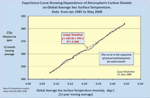
The late professor Lance Endersbee demonstrated that a straight line relationship exists with near perfect correlation between sea temperature versus CO2 concentration, which is consistent with Henry’s Law when time is de-seasonalized. http://icecap.us/images/uploads/Focus_0808_endersbee.pdf
Conclusions
Science observations and theory confirm that the atmospheric level of CO2 is always in balance with the sea surface temperature or else is dynamically moving through very large fluxes to re-establish that balance. CO2 emitted by humans from all sources is offset continuously by an equivalent amount of CO2 absorbed by the environment. In one geography, the net flux of CO2 gas is absorption into ocean surface while in another location the net flux CO2 is emission into air from the ocean surface. But in all locations, CO2 gas is simultaneously being emitted and absorbed since CO2 gas molecules are continuously colliding with ocean, plants, soil and all surfaces exposed to air. The ratio of absorption into the liquid surface versus emission from the liquid surface is the Henry’s Law constant, and it is specific to surface temperature, of the ocean, of a raindrop, of a bubble, of a leaf or alveolar tissue. The time derivative of the net CO2 concentration (i.e., the Keeling Curve, or slope, or rate of change of net CO2 concentration with respect to time) is specified in Fick’s 1st Law which is based on the surface area and surface thickness and gradient across that surface thickness at a given temperature and the diffusion constant (Graham’s Law). The time to recover from a perturbance to the Henry Law equilibrium is a function of the Law of Mass Action and Le Chatelier’s principle.
Important note: neither the amount of global human CO2 gas emissions nor the amount of global net human CO2 emissions (i.e., total human emission minus total absorption of human emissions) is measured by any agency; these are only estimated in models based dominantly on estimates of CO2 generated from a mixed bag of different fossil fuels and estimates offossil fuels production data submitted by countries. The uncertainty in these fossil fuel production data is significant (e.g. 15% from Mexico). The wide uncertainties in fossil fuels CO2 (FFCO2) are discussed in Bromley (2023) https://budbromley.blog/2023/05/25/un-ipcc-ar6-climate-report-apples-and-oranges/
“Despite its importance, the characterisation of uncertainty on estimates of the global total FFCO2 [fossil fuel CO2] emission made from the CDIAC database is still cumbersome…CDIAC has never published quantitative values for the uncertainty in national emissions, although many data users are aware that the uncertainty varies widely among countries.”…(page 1). Andres, Boden & Higdon (2014).
Uncertainty in estimated FFCO2 dwarf uncertainty in the gold standard measurement of net atmospheric CO2 concentration (specified as ~ 0.1 ppm in 400 ppm, or 0.025%. For MLO, “the reported uncertainty is the mean of the standard deviations for each annual period” (Conway et al.)
Estimates of human-produced CO2 emissions are trivially small:
The existing CO2 reservoir in air (about 700 gigatonnes) and the existing CO2 reservoir in ocean surface (about 1000 gigatonnes), and
trivially small with respect to the two continuous annual fluxes of CO2 gas (about 90 gigatonnes each) circulating back and forth between the atmospheric CO2 reservoir and ocean surface CO2 reservoir, and
Net human CO2 emissions for 2020 did not exceed 0.6% of net global CO2 for 2020. According to MLO for 2020, net CO2 from all sources and sinks, human and natural, on average increased only 2.58 ppm for the year 2020. That is only 0.000258% of the atmosphere and it includes all CO2 from all sources and sinks, natural and human. https://budbromley.blog/2022/11/01/about-those-errors-in-the-climate-change-gold-standard/
Emeritus Professor of Business, statistician Jamal Mushi, PhD, confirms in multiple papers and multiple tests that a statistical signal of the trend in estimated fossil fuel CO2 emissions is not detected in the trend of MLO-measured net global CO2. Munshi, J. (2017) “The essence of the theory of anthropogenic global warming (AGW) is that fossil fuel emissions cause warming by increasing atmospheric CO2 levels and that therefore the amount of warming can be attenuated by reducing fossil fuel emissions (Hansen, 1981) (Meinshausen, 2009) (Stocker, 2013) (Callendar, 1938) (Revelle, 1957) (Lacis, 2010) (Hansen, 2016) (IPCC, 2000) (IPCC, 2014). At the root of the proposed AGW causation chain is the ability of fossil fuel emissions to cause measurable changes in atmospheric CO2 levels in excess of natural variability.” Dr. Munshi, , reveals in his series of papers, the AGW argument is spurious and without merit because there is no correlation between the trend in estimated FFCO2 compared to the trend in measured net Mauna Loa CO2 emission.
Human emissions are rapidly absorbed by the environment. This is shown in Bromley & Tamarkin (2022). Professor Murry Salby highlighted the large scale of the difference between natural emissions and human emissions:
“Equally significant are transfers of carbon into and out of the ocean. Of order 100 GtC/yr, they exceed those into and out of land. Together, emission from ocean and land sources (∼150 GtC/yr) is two orders of magnitude greater than CO2 emission from combustion of fossil fuel. These natural sources are offset by natural sinks, of comparable strength. However, because they are so much stronger, even a minor imbalance between natural sources and sinks can overshadow the anthropogenic component of CO2 emission.”
“At an absorption rate of 100 GtC/yr, the ocean will absorb the atmospheric store of CO2 of 1000 GtC in about a decade. That absorption of CO2, which is concentrated in cold SST [Sea Surface Temperature] at polar latitudes, is nearly offset by emission of CO2 from warm SST at tropical latitudes. Warming of SST (by any mechanism) will increase the outgassing of CO2 while reducing its absorption. Owing to the magnitude of transfers with the ocean, even a minor increase of SST can lead to increased emission of CO2 that rivals other sources.” (3) M.L. Salby, 2012, p546.
A critically important point to understand is that the source of the CO2 is not a variable in Henry’s law phase-state equilibrium. Atmospheric CO2 concentration is not affected by humans but instead is controlled by natural chemical and physical processes which control CO2 gas solubility in all water in ocean, soil and biosphere. CO2 gas residence time in atmosphere and residual are irrelevant to the net CO2 atmospheric concentration, red herring distractions. Globally averaged, the other variables which affect local, immediate net CO2 concentrations cancel out, i.e., salinity, alkalinity, pH, air and water surface turbulence; globally these cancel out leaving surface temperature controlling the Henry’s Law constant for CO2 and water.
M. L. Salby, “Atmospheric Carbon”, Video Presentation, July 18, 2016. University College London. https://youtu.be/3q-M_uYkpT0.
M. L. Salby, “What is Really Behind the Increase of Atmospheric CO2“? Helmut-Schmidt-University Hamburg, 10. October 2018, https://youtu.be/rohF6K2avtY
M. L. Salby, “Relationship Between Greenhouse Gases and Global Temperature”, Video Presentation, April 18, 2013. Helmut-Schmidt-University Hamburg https://www.youtube.com/watch?v=2ROw_cDKwc0.
Stallinga, P. (2020) Comprehensive Analytical Study of the Greenhouse Effect of the Atmosphere. Atmospheric and Climate Sciences, 10, 40-80. Full paper in pdf here: https://www.scirp.org/pdf/acs_2020011611163731.pdf
Robert J. Andres, Thomas A. Boden & David Higdon (2014). A new evaluation of the uncertainty associated with CDIAC estimates of fossil fuel carbon dioxide emission.
“Coronavirus isolated from humans. “Patent No. US US7776521B1” Abstract: “Disclosed herein is a newly isolated human coronavirus (SARS-CoV), the causative agent of severe acute respiratory syndrome (SARS). Also provided are the nucleic acid sequence of the SARS-CoV genome and the amino acid sequences of the SARS-CoV open reading frames, as well as methods of using these molecules to detect a SARS-CoV and detect infections therewith. Immune stimulatory compositions are also provided, along with methods of their use.”
“This is a division of co-pending U.S. patent application Ser. No. 10/822,904, filed Apr. 12, 2004, and issued as U.S. Pat. No. 7,220,852 on May 22, 2007, which in turn claims the benefit of U.S. Provisional Patent Application No. 60/465,927 filed Apr. 25, 2003. Both applications are incorporated herein by reference in their entirety.”
“STATEMENT OF GOVERNMENT SUPPORT. This invention was made by the Centers for Disease Control and Prevention, an agency of the United States Government. Therefore, the U.S. Government has certain rights in this invention.”
By Martin Kulldorff, Biostatistician, Epidemiologist, Professor of Medicine, Harvard Medical School, Boston
Among COVID-19 exposed individuals, people in their 70s have roughly twice the mortality of those in their 60s, 10 times the mortality of those in their 50s, 40 times that of those in their 40s, 100 times that of those in their 30s, 300 times that of those in their 20s, and a mortality that is more than 3000 times higher than for children. Since COVID-19 operates in a highly age specific manner, mandated counter measures must also be age specific. If not, lives will be unnecessarily lost.
To determine effective public health counter measures against COVID-19, it is important to know the population characteristics of the epidemic [1]. It has been widely reported that mortality rates among those diagnosed and hospitalized are higher in older age groups [2, 3], but to determine public health action, it is the mortality among those exposed or infected that is of primary importance. Absolute risk estimates are uncertain at this stage of the epidemic, due to asymptomatic infected individuals [4] and limited population based testing [1], but with reasonable assumptions about exposure, it is possible to obtain rough estimates of the relative risks in different age groups, as well as upper bounds for the absolute risks.
We consider two alternative exposure scenarios at the early stages of the outbreak in Wuhan, before any social distancing was in place. In Scenario A, the likelihood of being exposed was equal in all age groups. In Scenario B, those <70 had twice the exposure compared to ages 70-79, who in turn had twice the exposure of those 80 and older. The truth probably lies somewhere in between these two scenarios.
Using Wuhan data for the relative risk of a COVID-19 diagnosis after exposure (RRC|E) and national Chinese data for the relative risk of death after a diagnosis (RRD|C) [2], the estimated relative risk of death among those exposed is RR = RRC|E x RRD|C. The Wuhan data better reflect the pre-social distancing phase of the epidemic while the Chinese mortality data increase the sample size of diagnosed individuals, generating more reliable estimates.
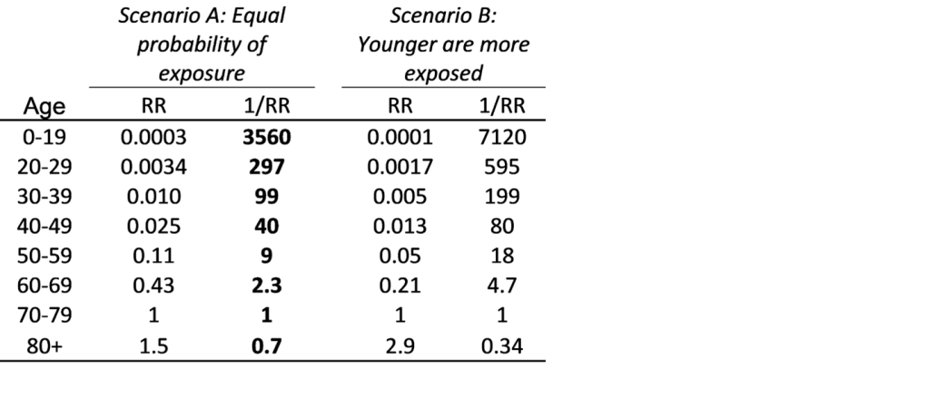
With age 70-79 as baseline, relative mortality risks are shown in Table 1. For COVID-19 exposed individuals, people in their 70s have roughly twice the mortality of those in their 60s, 10 times the mortality of those in their 50s, 40 times that of those in their 40s, 100 times that of those in their 30s, 300 times that of those in their 20s, and a mortality that is more than 3000 times higher than for children. Under Scenario B, with higher exposure among the young, the age differences are even larger.
In the United States, social distancing was in place early on, and since it is easier for retired people to stay home, it is likely that there was much less exposure among older people. Despite this, there is a higher proportion of diagnosed cases among the older population [5]. This means that the U.S. numbers are consistent with those from China.
Table 1: Relative risks (RR) for COVID-19 mortality by age group. In scenario A, pre-social distancing probability of exposure is assumed to be equal across all ages. In scenario B, it is assumed to be twice as high for those <70 and half as much for those >80, compared to age 70-79.
Since 1/RR is approximately 100 for age 30-39, exposure of only 1,000 people in their 70s would lead to the same number of deaths as the exposure of 100,000 persons in their 30s. In other words, in order to avoid the same fixed number of deaths, one must prevent COVID-19 exposure to 1,000 people in their 70s, or 10,000 people in their 50s, or 40,000 in their 40s, or 100,000 in their 30s, or 300,000 in their 20s, or 3.5 million children. Preventing exposure of 3.5 million children or 100,000 people in their 30s is practically, logistically, and financially more challenging than preventing exposure of 1,000 people aged 70-79.
Government officials would be wise to take advantage of these widely different mortality rates by age in devising their COVID-19 counter measures, while still maintaining essential societal services. Whether mandated counter measures are intensified, recalibrated, or gradually relaxed sometime in the future, age specific measures should be part of the strategy. If not, there will be unnecessary mortality, burden on hospitals and economic disruption. Counter measures directed specifically at older people will not only protect them, it will also free up health care resources for those younger people that do need hospital care.
To date, most government mandated mitigation measures have either been age neutral, such as restaurant closures, or targeted at young and middle-aged people, such as school and office closures. A more appropriate age targeted approach is needed. Just as some pubs ban customers under the age of 21, government officials could set temporary upper age limits of say 50, 60, or 65 for visiting or working at restaurants, stores, offices, airports, and other public places. So, for example, while all 60-plus-year-old supermarket cashiers, gas station attendants, police officers, postal workers, garbage collectors and bus drivers should stay home, their younger colleagues should keep working, taking extra shifts as needed.
Counter measures must consider not only relative risks but also absolute risks. Among diagnosed cases age 70-79, the mortality rate in China was 1 in 25. [2] Their absolute mortality risk when simply exposed is then less than that, although we do not know how much less. Transformed to other age groups, using the data from Table 1, the absolute risk-of-death point estimates among those exposed is less than 1 in 25×3560=89,000 for children, less than 1 in 7,500 for age 20-29, less than 1 in 2,500 for age 30-39, less than 1 in 1,000 for age 40-49, less than 1 in 230 for age 50-59, less than 1 in 58 for age 60-69, less than 1 in 25 for age 70-79 and less than 1 in 17 for those in the 80+ age group. These numbers for exposed individuals are more favorable but similar to recent mortality estimates for infected individuals [3]. To put these upper bounds in context, the upper bounds for children and young adults are lower than the U.S. infant mortality rate of 1 in 170 or the annual child mortality rate of around 1 in 6,000 [6]. For the older age groups, on the other hand, the upper bounds on the mortality rates are staggeringly high.
Infectious disease outbreaks have occurred throughout history and will continue to do so, aided by urbanization and long-distance travel. COVID-19’s ability to kill and its rapid spread make it a formidable enemy that is impossible to stop until herd immunity is reached. Just as in war, we must exploit the characteristics of the enemy in order to defeat it with the minimum number of casualties. Since COVID-19 operates in a highly age specific manner, mandated counter measures must also be age specific. If not, lives will be unnecessarily lost.
Martin Kulldorff, Biostatistician, Professor of Medicine, Harvard Medical School, Boston
References
[1] M. Lipsitch, D. L. Swerdlow och L. Finelli, ”Defining the Epidemiology of Covid-19 — Studies Needed,” New England Journal of Medicine, vol. 382, pp. 1194-1196, 2020.
[2] J. T. Wu, K. Leung, M. Bushman, N. Kishore, R. Niehus, P. M. d. Salazar, B. J. Cowling, M. Lipsitch och G. M. Leung, ”Estimating clinical severity of COVID-19 from the transmission dynamics in Wuhan, China,” Nature Medicine, pp. 1-5, 2020.
[3] R. Verity, L. C. Okell, I. Dorigatti, P. Winskill, C. Whittaker, N. Imai, G. Cuomo-Dannenburg och etal, ”Estimates of the severity of coronavirus disease 2019: a model-based analysis,” The Lancet Infectious Diseases, 2020.
[4] R. Li, S. Pei, B. Chen, Y. Song, T. Zhang, W. Yang och J. Shaman, ”Substantial undocumented infection facilitates the rapid dissemination of novel coronavirus (SARS-CoV2),” Science, nr March 16, 2020.
[5] CDC COVID-19 Response Team, ”Severe Outcomes Among Patients with Coronavirus Disease 2019 (COVID-19) — United States, February 12–March 16, 2020,” Morbidity and Mortality Weekly Report, vol. 69, nr 12, pp. 343-346, 2020.
[6] S. L. Murphy, J. Xu, K. D. Kochanek och E. Arias, ”Mortality in the United States, 2017,” National Center for Health Statistics, Hyattsville, MD, USA., 2018.
If we take human-caused global warming (AGW) as analogy, most of the world is already awakened to the fact that AGW is a fraud. For example, AGW is at the bottom of the list of concerns in surveys by the WHO. But WHO/UN management has AGW as a top priority as do over 100 governments.
AGW and pandemic fear mongering will stay as top priority for governments so long as voters continue electing politicians whose campaigns are funded by these special interests. AGW has been a political issue for over 30 years now, even though tens of thousands of scientists and thousands of peer review publications refute the AGW fraud.
Similarly, this virus “pandemic” is not about the science or disease, just as AGW is not about the science or the environment. Both are about politicians and government taking more control over people and resources; these are regressive political strategies, though supported by so-called “progressives,” promoted by revolutionaries and the communist/collectivist ideology to empower government control of everything. It will continue until voters throw them out of office.
Dr. Ryan Cole, pathologist, in the video at the link above essentially confirms the results of autopsies by pathologist Dr. Peter Schirmacher in Germany.
Dr. Peter Schirmacher, German pathologist, performed autopsies on 40 people who had died within two weeks of receiving a covid jab. Of those he autopsied, 30%-40% could be directly attributed to the “vaccines.” ‘In his opinion, the frequency of fatal consequences of vaccinations is underestimated…’ Dr. Schirmacher is world-renowned in his field, honored by The Pathologist as one of the 100 most influential in the world. He is the acting chairman of the German Society of Pathology, director of the Institute of Pathology at Heidelberg University Hospital, and president of the German Association for the Study of the Liver.
by Professor Hermann Harde, Experimental Physics and Materials Science, Helmut-Schmidt-University, Hamburg, Germany
Abstract: (link to full paper below. Published June 12, 2019)
The Intergovernmental Panel on Climate Change assumes that the inclining atmospheric CO2 concentration over recent years was almost exclusively determined by anthropogenic emissions, and this increase is made responsible for the rising temperature over the Industrial Era. Due to the far reaching consequences of this assertion, in this contribution we critically scrutinize different carbon cycle models and compare them with observations. We further contrast them with an alternative concept, which also includes temperature dependent natural emission and absorption with an uptake rate scaling proportional with the CO2 concentration. We show that this approach is in agreement with all observations, and under this premise not really human activities are responsible for the observed CO2 increase and the expected temperature rise in the atmosphere, but just opposite the temperature itself dominantly controls the CO2 increase. Therefore, not CO2 but primarily native impacts are responsible for any observed climate changes.
Hermann Harde, What Humans Contribute to Atmospheric CO2: Comparison of Carbon Cycle Models with Observations, Earth Sciences. Vol. 8, No. 3, 2019, pp. 139-159. doi: 10.11648/j.earth.20190803.13
I will also post here links to all of the materials he mentions on the thumb drive.
This is about 5 minutes and fast paced. His presentation was 7 August 2021. Entire board meeting (1 hour) is also recorded. In case you want this context, please let me know.





You must be logged in to post a comment.