Pinatubo Study Phase 1 Report

By: Bud Bromley, April 29, 2022

Contributing Editor:  Tomer Tamarkin

Abstract

Digital signal processing technology was used to analyze daily carbon dioxide data from the joint NOAA – Scripps Oceanographic Institution’s Global Monitoring Laboratory (MLO).  The period surrounding the 1991 eruption of the Pinatubo volcano was rigorously analyzed for slope and acceleration of net global average atmospheric CO₂ concentration and found to be consistent with the theory that Henry’s Law, the Law of Mass Action, and Le Chatelier’s principle control net global average atmospheric CO₂ concentration rather than human-produced CO₂ emissions.  Background and theory are explained.  A method of using common physics and math for a novel purpose is presented to compare natural CO₂ emission or absorption with human-produced CO₂ emission.  The claim that human-produced CO₂ emission is causing increasing global CO₂ concentration and climate change is shown to be without scientific merit.  

Key words: carbon, CO₂, climate, warming, Impulse, Pinatubo, Henry’s Law, Mauna Loa 

Introduction

William Henry tested and documented his series of experiments on different gas and liquid combinations under various conditions which were published in 1803. (Henry, 1803)   Today, the coefficients he developed are now available in tables in reference books and software which are used routinely by chemists and chemical engineers.  This stable science is known today as Henry’s Law and is a foundation science for several large industries.  Though it is not common knowledge among the public and only rarely found in climatology literature, Henry’s Law is the fundamental science for the multi-billion dollar per year scientific instrumentation industry of gas chromatography, which is one of the methods used to measure atmospheric gases and most chemicals.  It is also a fundamental science underlying chemical engineering in gas, oil and coal refining and the beer and carbonated beverage industries.   Also, it is one of the major variables in the absorption and emission exchanges of oxygen and carbon dioxide and other gases in the lungs and gills of all animals. 

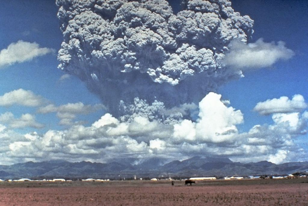
The Pinatubo eruption pictured in Figure 1 and its causes and effects are the subjects of many studies, for example, Stenchikov (2021).   

An excerpt from Science News at the time from Hoppe (1992):

Ellsworth G. Dutton, a meteorologist with NOAA’s Climate Monitoring and Diagnostics Laboratory in Boulder, Colo., traced the effects of Pinatubo’s cloud with ground-based instruments that directly measure the strength of sunlight. Dutton says his results show a 20 to 30 percent decline in the amount of solar radiation that reaches the ground without being scattered or reflected, and a 2 to 4 percent decline in total solar radiation.

Temperatures have already started to drop, both at ground level and in the lower atmosphere, says James K. Angell of NOAA in Silver Spring, Md. Angell told Science News his analyses of weather balloon data show that the first half of 1992 was 0.4 [degrees] C cooler, overall, than the first half of 1991. He notes that the volcano’s effect may be greater than suggested by these observed temperature shifts, since this year’s El Nino warming would normally raise average temperatures by 0.2 [degrees] C (SN: 1/18/92, p.37).

Weather satellites confirm cooling in the lower atmosphere, recording a global drop of more than 0.5 [degrees] C since last June, with this June being 0.2 [degrees] C cooler than average, according to John Christy of the University of Alabama at Huntsville and Roy Spencer of NASA’s Earth Science Lab at the Marshall Space Flight Center in Huntsville. Christy says their data indicate that the greatest cooling, 1.0 [degrees] C, occurred in the northern midlatitudes — an area that includes the continental United States — while temperatures in the southern hemisphere have dropped by only 0.3 [degrees] C.

Figure 2 from the Mauna Loa Observatory shows reduced atmospheric transmission of solar radiation due to volcanic aerosols after the Pinatubo volcanic eruption.

Pinatubo was the largest or second largest volcanic explosion observed on Earth in the last 100 years.  The explosion resulted in a belt of clouds, dust, various gases, and particles encircling and spreading in the atmosphere around Earth’s tropical zone, which is about 20 degrees latitude both north and south of the equator.  In this large zone, ocean surface temperature averages 25 degrees C (77 degrees F) year-round, in contrast to average ocean temperature of 17 degrees C.  Figure 3 shows the large negative change in temperature after the Pinatubo eruption.

On average, ocean surface above 25 degrees C or 298.15 Kelvin is a net emitter of CO₂ gas, day and night, year-round.  That is, more CO₂ is being released from ocean surface than is absorbed from among the CO₂ molecules which are continuously colliding with the ocean surface.  (25 degrees C is not a set point like a boiling point. It is a standard agreed by standards organizations, part of Standard Ambient Temperature and Pressure (SATP). The belt of clouds, gases, and particles, etc., encircling the tropics is assumed by all known reports to have reduced short wave solar insolation reaching the surface; incoming sun light around 400 to 700 nanometer wavelength was shaded, blocked, absorbed, reflected, scattered, or otherwise obfuscated.  Consequently, tropical ocean surface cooled.  Higher latitude ocean surface cooled also. 

Our theory is that Henry’s Law controls net global average atmospheric CO₂ concentration and human CO₂ emission only temporarily perturbs net global average atmospheric CO₂ concentration and its rate of change. There are knowledgeable groups of scientists, such as chemists, analytical chemists, and chemical engineers, as well as individual scientists in other fields who support this theory.  But this theory is rarely studied or found in climate literature and rarely funded in government environmental work.  Generally, papers concerning Henry’s Law and climate are found only in less well-known journals.

Henry’s Law is a reproducible, well-documented law of chemistry and physics which defines the ratio of any gas in contact with any liquid.  Each gas and liquid combination has a specific Henry’s Law coefficient, herein denoted k_H.   The coefficient is not a constant; k_H varies with temperature at the gas – liquid interchange surface. Concentration of CO₂ (g) in seawater is inversely proportional to sea surface temperature.  

The Henry’s Law phase-state equilibrium equation can be rearranged and derived for several different important applications, for example, solubility or volatility. As used here, k_H is ratio of the moles of aqueous-phase CO₂ gas per mole of water versus the moles of gas-phase CO₂ gas per mole of air above the water surface. This resulting partition ratio, known as the Henry’s coefficient ratio is dimensionless, i.e., without units. As used here k_H is the same as H^scc or H^cc in Sander (2015).

k_H = [CO₂(aq)] / [CO₂(g)] is dimensionless and temperature dependent.  (1)

Henry’s Law has limitations on its application.

1. Henry’s Law only applies when the concentration of the unreacted gas in the liquid is minor and when the concentration of gas being measured in the gas volume above the liquid (i.e., its partial pressure) is minor relative to the other gases in the volume.  An oversaturation condition is observed in chromatography by an abnormal, non-Gaussian peak shape.  Henry’s Law is applicable to CO₂ gas since it is a trace gas in both the atmosphere and in the ocean even at 10 times current concentrations.    

2. Henry’s Law only applies to the gas in the liquid which has not reacted with the liquid; that is, Henry’s Law only applies to the reversible phase-state equilibrium reaction [CO₂(g)] <-> aqueous [CO₂(g)].  Henry’s Law does not apply to ionized CO₂ gas, that is, hydrated CO₂, nor to any of the carbonate or bicarbonate ions or un-ionized carbonic acid that are products of aqueous CO₂ gas known collectively as dissolved inorganic carbon (DIC).

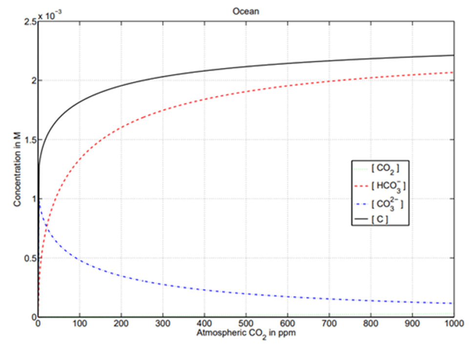
The total concentration of dissolved inorganic carbon from Cohen and Happer (2021):

[C] = [CO₂] + [HCO^{− 3}] + [CO₂^{− 3}] (2)

After the hydration of CO₂(aq) in acid-based reaction with water ions, the solubility coefficients of the subsequent species vary with (a) temperature of the surface (b) salinity of the liquid including certain minerals which are dissolved in the liquid not only sodium chloride, (c) alkalinity or pH or the liquid, (d) partial pressure of the gas in the space above the liquid and (e) partial pressure of the gas in the liquid.  High diligence is needed in sampling procedures to control (a), (b), (c), (d) and (e). 

Most of the CO₂ in seawater is in DIC form, which, according to most estimates, is on the order of 38,000 gigatonnes (Gt) of DIC dissolved or reacted in deep seawater. Meanwhile 1000 Gt of DIC is estimated to be in surface seawater and 850 Gt in air. (One Gt is 1000 billion kilograms, that is, 1 followed by 12 zeros, or 1 X 10¹² kilograms).  Figure 4 below (Cohen & Happer, 2021) illustrates the relative molar stoichiometric concentrations of the DIC species in ocean corresponding to atmospheric CO₂ concentration. Barely visible, the fine dotted green line slightly above the horizontal axis is increasing. The concentration of the CO₂(aq) species of DIC in ocean and the concentration of the bicarbonate species in ocean are both increasing as atmospheric CO₂ concentration increases.  Simultaneously, the carbonate ion [CO₂^{− 3}] of carbonic acid is decreasing, along with alleged problems of so-called “ocean acidification”.

Average ocean water is above pH 8, which means ocean is alkaline, not acidic. For example, if pH were to change to 7.9, then the ocean is not more acidified because at 7.9 there is an excess of alkaline ions to neutralize acid ions, thus ocean is simply less alkaline. Ocean acidification is a misnomer.  

Since no alternative CO₂ sink of sufficient size or rate is known, then CO₂ gas must be rapidly absorbed into sea surface when the surface cools.  Ocean surface demonstrates the capacity to rapidly absorb orders of magnitude more CO₂ than humans produce, and then recover to trend. It is imperative to recognize that these reactions of ionized CO₂ (DIC) are rapidly reversible reactions. In the following discussion, we do not rely on estimates or models of CO₂ in air and seawater to demonstrate this point.

Aqueous CO₂(g) <-> H⁺ + HCO₃^– (3)

Most CO₂ in seawater is in the ionized form HCO₃^– known as bicarbonate as shown above in figure 4 (Cohen & Happer, 2021).  Minor changes in ocean surface temperature reverse the CO₂ hydration reaction and aqueous CO₂ gas is formed.  Colder water pushes this reaction to the right, to products.  Warmer water pushes the reaction to the left, to reactants. Once in its aqueous CO₂ gas state, then the Henry’s Law dynamic equilibrium applies: for a given seawater surface temperature, there is a fixed ratio of CO₂ gas concentration in air versus CO₂ gas concentration in seawater surface which is in contact with the air.  Depending on changes in surface conditions, aqueous CO₂ gas could react with H₂O to become H₂CO₃ (carbonic acid), or it could react with H₂O to become HCO₃^– (bicarbonate) plus hydrogen ion (hydronium), or it could remain in the water matrix as aqueous CO₂ gas, or it could be emitted to the atmosphere as CO₂ gas.  

Cohen and Happer (2021) point out that transition of only a single proton (a hydrogen ion), determines bicarbonate versus carbonic acid species.  The various DIC species are surrounded in the seawater matrix by hydrogen ions and hydroxide ions.  CO₂ gas molecules and DIC ions are not required to move in the seawater matrix.  Both bicarbonate ion and carbonic acid are separate reaction products of the aqueous CO₂ gas hydration reaction with H₂O, as well as reversible with each other, as shown in the next graphic.  In seawater surface these reactions can reverse in seconds due to changing surface temperature, or agitation by waves, buoys and moving ships, or a sampling procedure, or by an upwelling water current dense with DIC (e.g., an El Nino current).  As upwelling seawater dense with DIC comes to the surface, it warms, and aqueous CO₂ gas in the surface becomes oversaturated, out of balance with the Henry’s Law ratio for the temperature at the surface, resulting in CO₂ gas being emitted to the air and a rebalancing the Henry’s Law dynamic equilibrium for that temperature. 

Professor Daniel Mazza explains reversible reactions of higher order (Mazza, 2020, pp16-17):

 At any given temperature, the value of Keq remains constant no matter whether you start with A and B, or C and D, and regardless of the proportions in which they are mixed. Keq varies with temperature because k1, and k2 vary with temperature, but not by exactly the same amount. 

… the general formulation of the law of mass action (Guldberg-Waage, 1864) that states: in a chemical system at equilibrium and constant temperature, the ratio between the product of the concentrations of chemicals formed (each elevated to its stoichiometric coefficient) and that of the reagents is a constant value.

The reactants and products of the carbonate chemistry in seawater are difficult to sample and quantify with precision because the reactions are so rapid and only very minor changes in surface conditions are required to change the dynamic equilibrium by increasing the ocean surface area in contact with air. Taking a sample affects the reactions. Special methods and systems must be used for these analyses at the thin layer at ocean surface.  Journal and online articles report years or hundreds of years are required to move large amounts of CO₂, allegedly because migration of CO₂ vertically or horizontally in the water matrix is slow.  There are such slow changes, with El Ninos and La Ninas being prime examples. However, simultaneously, second by second, bulk CO₂ gas is continuously in flux into and out of millions of square kilometers of ocean surface, driven by SST change and CO₂ is converting in seconds from one ionic species to another and aqueous CO₂ gas is either released to air or hydrated to carbonic acid or bicarbonate.  Additional data experiments will probably reveal that slower or continuous changes such as human emissions are anomalous perturbations to the trend of the dynamic equilibrium for the local surface temperature.  Adding or subtracting CO₂ from any source or for any residence time or emission rate does not change the Henry’s ratio for a given temperature.                  

Demonstrating an example of this bulk sea surface reaction and its enormous quantity and rate in the natural environment as observed in the Mauna Loa data is a primary objective of this study.        

Note that the hydration reaction of aqueous CO₂ gas with H₂O, (3) in Figure 5, is cyclical. Each reaction (1), (2) and (3) is reversible. The forward (left to right) and reverse direction (right to left) are not equal in each of the three reactions.

Changes in kinetics force the reactions forward or backward. Changes in kinetics are changes in motion of molecules.  Agitating the surface of the ocean warms the water, which changes the Henry’s Law ratio, increases the partial pressure of CO₂ gas in ocean surface. Those kinetic changes result from heating, cooling or agitation of the sea surface by waves, ships underway and buoy motion, currents, storms, gas and water sampling procedures, etc.  For example, warm tropical sea surface that is normally continuously emitting CO₂ gas can be depleted of CO₂ gas by wind, storms, hurricanes, typhoons, etc. with the result that the undersaturated sea surface is subsequently absorbing CO₂ from air instead of emitting.  Significant sampling problems in actual sea water include CO₂ gas added or subtracted by the biology – living and dead – in the sea, currents of seawater dense with CO₂ upwelling from deep ocean to the surface, and sampling sea surface when the necessary representative sample is only the top centimeter or less thin layer.        

Simultaneously with the portion of the carbonate chemistry described above, calcium ions (Ca²⁺), which are readily available in seawater in great excess to carbon, react with bicarbonate ions (HCO₃^–) producing calcium carbonate (CaCO₃).  This reaction is not included in the Henry’s Law equilibrium, and not included in the estimated 38,000 Gt of DIC, and not included in the estimated 1000 Gt of DIC in sea surface, although it is accumulated inversely proportional to temperature into the largest CO₂ sink by orders of magnitude. Richard E. Zeebe and Dieter A. Wolf-Gladrow remind us, aqueous CO₂ gas as well as solid precipitant calcium carbonate are produced, “at surface water conditions… counterintuitively.. during CaCO₃ precipitation CO₂ is liberated…by only ~0.03 µmol per µmol CaCO₃ precipitated.” (Zeebe & Wolf-Gladrow) The famous white cliffs of Dover and Sussex, England, limestone caves around the world, the famous marble quarries of Italy are examples of enormous CaCO₃ deposits.  Ultimately, when aqueous CO₂ is oversaturated with respect to the Henry’s ratio, the Law of Mass Action requires the DIC and Ca²⁺ reactions to move to the right, towards products; thus excess CO₂ is converted to one of the forms of calcium carbonate. The calcium carbonate precipitates as solid particles which sink in the ocean water column, removing it from the surface layer. The calcium reaction is another source of CO₂ in sea water while at the same time it removes bicarbonate from seawater.

Ca²⁺ + 2HCO₃^– -> CaCO₃ + CO₂ + H₂O  (4)

CO₂ dissolved in ocean surface is estimated to be 30 to 40 times more concentrated than in air, resulting from multiple reactions, yet still a minor component of sea surface water. But, these estimates of CO₂ in ocean surface include ocean surface that is many meters deep.  In this report, we are concerned with the CO₂ in the thin layer at the sea-air interface.  This report and project do not rely on estimates of CO₂ concentration, nor on estimates of ocean layer thickness.  Demonstrating measurements of CO₂ absorption and emission and their rates in comparison to human emissions is the purpose of this project.

Additional background on Henry’s Law and the carbonate chemistry is found in, for example, Cohen and Happer (2021), Stallinga and Khmelinskii (2018), Stallinga (2018), Harde (2019), Zeebe and Wolf-Gladrow, and Mazza (2020).    

Our theory is net global atmospheric CO₂ concentration is in a dynamic equilibrium that is constantly re-balancing CO₂ concentration between atmosphere and ocean surface, a re-balancing based primarily on the change in relative surface area of Earth and SST. Flux is not the same as flow or flow rate.  Flux is the mass flowing through a 2 dimensional area per unit of time (e.g. grams per square meter per second, or gigatonnes per square meter per hour, etc.). Flow rate is the volume of moving in a unit of time (e.g. liters per minute, gallons per hour, cubic meters per hour, cubic feet per second, etc.). Sea surface temperature (SST) and surface area at SST must be used to calculate CO₂ flux. Average ocean temperature or average air temperatures or average SST result in incorrect Henry’s law equilibrium calculations. The Henry’s Law phase-state equilibrium reaction is diffusion of un-ionized CO₂ gas through a surface area, that is, a two-phase equilibrium which is dynamically mediated by local SST and relative surface area at SST. At equilibrium, the resulting concentration gradient of the CO₂ solute between the two sides of the exchange surface is the Henry’s Law dimensionless ratio. Equilibrium at a given surface temperature does not imply that the two fluxes are equal. Equilibrium at a given surface temperature implies that the ratio of net mass transfer in opposite vector directions through the given surface area is the dimensionless Henry’s Law coefficient for the given SST.

CO₂ gas is always being emitted from ocean surface and always being absorbed into ocean surface. CO₂ gas molecules never stop colliding with the ocean surface. Collisions result in increased kinetic energy in ocean surface followed by emission of CO₂ gas from the surface because the partial pressure of CO2 gas in the surface is increased by the collisions. Many factors affect ocean surface temperature in addition to insolation; insolation is a very important topic but well beyond the scope of this paper.  In higher latitudes, millions of square kilometers of ocean surface are usually at ~17 degrees C or less, year round, and in this area of ocean surface net absorption of CO₂ gas exceeds net emission, year round. Simultaneously, millions of square kilometers of tropical ocean are generally above ~25 degrees C year round, and in this area of ocean surface, net emission of CO₂ gas exceeds CO₂ absorption, year round.

Method

The first phase of this study sought to determine if we could detect, in the “gold standard” data for global CO₂ concentration, an inflection point in the slope of the daily CO₂ concentration measurements before, during or after a single major climate event, the explosive volcanic eruption of Pinatubo on the island of Luzon in the Philippines in June 1991.  Proprietary software for digital signal processing was used to analyze the publicly available daily CO₂ concentration data reported by MLO.  We defined an inflection point as a change in sign of the slope of CO₂ concentration after the eruption of Pinatubo.  Hypothetically, if we are able to detect these inflection points with statistical confidence, then, to support our theory, we can use the same data set and software to produce evidence from many different climate, weather and environmental events and a global CO₂ calibration curve. We would be able to measure changes in CO₂ concentration which resulted from other volcanoes, El Ninos, La Ninas, storms, human CO₂ emissions, and other events which reportedly affect net global average atmospheric CO₂ concentration.  In a sense, we are iterating William Henry’s experiments for CO₂ gas and water at the global scale with various climate and environmental conditions but using only measured global data.  Instead of unreliable computer climate models with too many estimates and theories, we would have data experiments using empirical data from the natural environment to correct the pervasive misunderstanding of CO₂ which is curated in popular culture and education. 

The MLO data was selected because it is widely recognized and reported to be the gold standard reference measurement for net global average atmospheric CO₂ gas concentration.  The lab is located about 11,000 feet above sea level on the northwest facing flank of Mauna Loa volcano on Hawaii island, the Big Island of Hawaii.  This data set was selected because it is accessible to the public and it has been diligently measured and curated since the 1970s. We selected their set of daily CO₂ measurements. The data are reported in micromoles of CO₂ gas per mole of dry air, which is equal to parts per million (ppm) CO₂ in dry air.  We are grateful to the MLO scientists, authors and administration for making these data available to the public (See acknowledgments and Thoning et al (2021) reference for details and access to the data).

The software toolset for this initial phase of the study was designed and operated by Shahar Ben-Menahem, PhD (physics, Stanford) and Abraham Ishihara, PhD (Aeronautics & Astronautics, Stanford) through their company Modoc Analytics LLC under contract with EnergyCite (https://energycite.com/) and its sister company ClimateCite (https://climatecite.com/)

Using these software tools, if these data were found to be responsive to a geographically remote event such as Pinatubo, then potentially it would not be necessary to examine many different CO₂ data sets nor to employ laboratories to validate our theory.  Instead of relying on theory, we would have measured, empirical evidence that CO₂ concentration is controlled by nature. Our theory assumes sea surface temperature (SST) directly affects the ratio of atmospheric CO₂ gas concentration versus CO₂ gas concentration in sea surface, following Henry’s Law, while human CO₂ has no effect on that ratio.  

Care must be taken with Henry’s Law since it can be expressed in many forms for different uses.  Here we use its dimensionless form.  The Henry’s Law coefficient k_H = c(aqueous)/c(gas) where c is concentration in moles.  For example, 400 micromoles of CO₂ per mole of air (which is 400 ppm CO₂ concentration in air) is in equilibrium with 333 micromoles of CO₂ per mole of seawater in sea surface at 298.15 K (or 25 degrees C) and a solution density of 997 kg/m³.  Dimensionless k_H = 0.8317 (Sander, 2015). Concentration of CO₂ in seawater is directly proportional to depth due to higher density (kg/m³) and inversely proportional to temperature. 

If this first phase data experiment worked, then the overall scientific complexity, effort, and expense of our project would be greatly reduced.  The most difficult data experiment was done first: could we detect the Pinatubo perturbation in the MLO data? 

We calculate a not-to-exceed amount of human-produced CO₂ based on measured data rather than assuming estimates of human-produced CO₂ based on estimates of fossil fuel production and cement production from spurious and dubious sources.  This is not to doubt the diligent and careful curation of the data by Oakridge National Laboratories, for example.  But the data they are handed comes from some sources which have been dubious over the years, for example, Soviet Union, Nigeria, Iran, Venezuela, and OPEC.   

This first phase of our project analyzed daily CO₂ data from MLO to determine if the changes in CO₂ due to the Pinatubo eruption were measurable in the data.  Is the data set responsive to remote events?  Could the software and skills of our scientists detect a reduction in the CO₂ concentration and an inflection point in rate of change of concentration due to cooling of tropical ocean surface by the Pinatubo cloud belt.  Velocity and acceleration of net global average CO₂ concentration were calculated based on measurements.    

The raw daily MLO data (as raw as available publicly) from the 1970s through 2020 was used as input for our sequence of algorithms. This “raw” time-series data set was only changed by us to fill in days with missing data.   

Data for days for which no real CO₂ data were available from MLO, marked as 999 in the MLO data file, but for which data were available for days both preceding and following the block of missing-data day(s), were interpolated accordingly.

Data for days (at the beginning of the recording period — early 1970s) for which no real data were available and no earlier data with valid data were available — were replaced by constant nominal values in the low 300s. This block of data is limited to the early 1970s and does not affect our Pinatubo results.

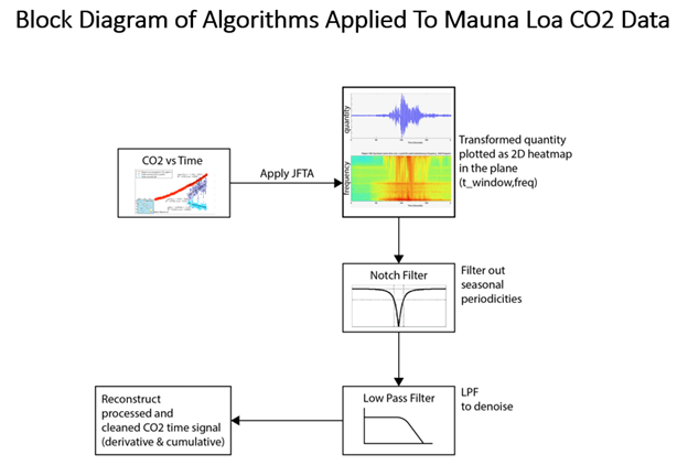
The following mathematical procedures (as summarized by boxes in the block diagram Figure 6.) are then applied to this “raw CO₂ level data” time series wherein time is given in fractional Gregorian years and CO₂ levels are given in ppm. 

A JTFA (“Joint Time Frequency Analysis”) is performed. Those skilled in the art of time-series digital signal processing (DSP) will recognize that this term refers to a class of methods, wherein a quantity-vs-time series is analyzed for its frequency content (such as PSD = Power Spectrum Density) as a function of time. While there are many JTFA techniques, the simplest one is performing a Fast Fourier Transform analysis (FFT) in a moving (“swept”) time window and computing the complex FFT coefficients as a function of both window start-time and in-window frequency index. This type of JTFA transformation, however, is not easily invertible.   

One of the simplest sub-classes of JTFA methods which is easily invertible, is the Gabor Transform.  The Ben-Menahem- Ishihara proprietary analysis method used in this investigation was based on combining the Gabor Transform and FFT.   

In the quantity-vs- time-frequency analyzes raw data result of our JTFA, we then remove the seasonal (1-year period) frequency-band peak via a notch filter, and also suppress the high-frequency band (“low-pass filtering”). Those skilled in the art of DSP or analog filtering in electrical engineering and other branches of physics-based engineering will readily recognize these terms and techniques.

After the notch- and low-pass filtering of the JTFA-produced data — represented by the relevant boxes in the Block Diagram — the filtered JTFA transform is then inverted. This computation yields the output (lower-left) box of the Block Diagram — the processed CO₂ vs. time signal (and its time derivative).

Then with these data we introduce a proven and well-known math and physics calculation to compare natural CO₂ absorption into the environment with human emissions.  

Results:

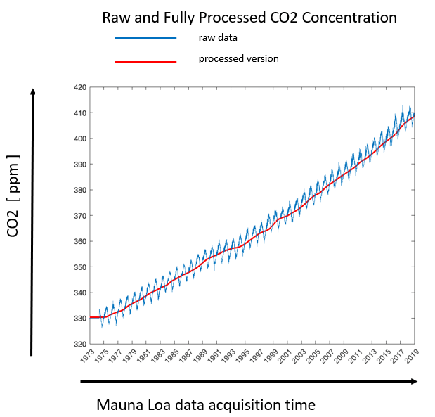
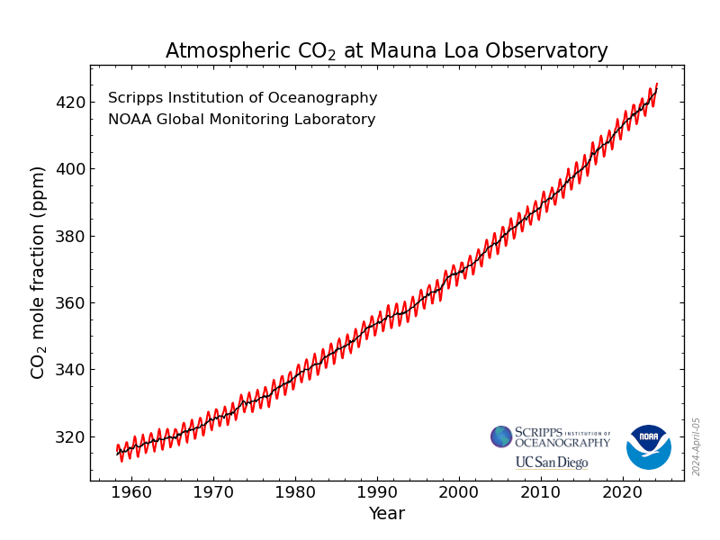
The graph in Figure 7 above is plotted over the entire Mauna Loa recording epoch (circa 5 decades) with both the “raw” (as defined above) and processed (as defined above) CO₂ levels, vs. time.  The graph appears very similar to the graphs typically produced by NOAA which appear frequently in media, education, politics and online. 

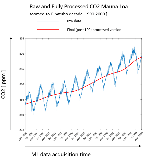
The graph above in Figure 8 is processed as in the previous graph in Figure 7 and described in the method section above but simply zoomed in to cover only the Pinatubo decade: 1990-2000. The slope of the red line is visibly bending or flattening in July of 1991 into 1994, and then in 1995 the slope turns upward again.

The data in the graph Figure 9 above is again processed as the previous two graphs but here zoomed in to the year of Pinatubo plus the year before and after Pinatubo.  The slope (grey line) is slightly bending or flattening after mid-year 1991 when the Pinatubo eruption occurred.  Velocity of CO₂ concentration is slowing after mid-year 1991.  

No inflection point in the slope of CO₂ concentration was found in the period following the Pinatubo eruption.  Slope declined slightly from prior trend but did not turn negative.  Large changes in acceleration were detected.  In this case, acceleration is the rate of change of slope, or the time derivative of CO₂ ppm per year.      

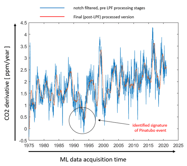
The graph in Figure 10 above plots the time derivative of the processed CO₂ ppm/year. These data provide the maximum deceleration and date, and the maximum acceleration and date, and concentration in ppm per year at those dates in the post Pinatubo period. From these data points, we calculated CO₂ flux and average mass of CO₂ that we suggest was diffused through ocean surface.

The above plot in Figure 11 is the time derivative of the processed CO₂ ppm/year.  The estimated “would-be inflection” times bracket the detected “Pinatubo Event” as indicated by arrows and DD/MM/YY date markers.  The bracket dates are the points of fastest decline (deceleration) of slope and the fastest increase (acceleration) of slope.  On this plot, the mean baseline pre- and post-Pinatubo CO₂ slope are indicated as horizontal lines; the full time period of the Mauna Loa data before or after the “would-be inflection” times were used to calculate the means, 1970s to 2020.  The points of minimum and maximum acceleration are used to determine respectively the end point of the pre-Pinatubo mean and the start point of the post-Pinatubo mean.  These two points allow assignment of the points where offset is calculated.  This offset (or over-recovery) is expected based on Le Chatelier’s Principle, basically stated, a perturbed trend will rapidly return to its equilibrium condition plus an offset amount or overcorrection. That is, the slope of the Henry’s phase-state equilibrium reaction for CO₂ does not recover to the previous pre-Pinatubo slope, but instead, it recovers to the slope that would have existed if the disturbance to the slope had not occurred. This strongly suggests that the rate itself (i.e., the Henry’s partition coefficient) is the controlling variable.

Discussion:

Now we have a reliable method based on gold standard measurements of a single climate variable, i.e. net global average atmospheric CO₂ concentration from MLO, which we can use to compare human-produced-CO₂ emissions with changes in net global average atmospheric CO₂ concentration. 

The trace gas CO₂ is produced, modified, and absorbed through many and varied natural processes in the environment.  Documenting and quantifying all of these with accuracy and precision into a so-called carbon budget or energy balance is a quixotic task and approximate at best, yet that is what the public through their governments are paying for in elaborate projects, for example, annually documenting Earth’s carbon balance in over 100 pages by dozens of authors, e.g., Friedlingstein (2021), not to mention United Nations Intergovernmental Panel on Climate Change (IPCC) climate conferences around the world and their thick document and public relations campaigns. It is a climate modeler’s dream project with no end date and expanding budgets.  These reports use too many estimates in too many models, not measurements of human-produced CO₂.   

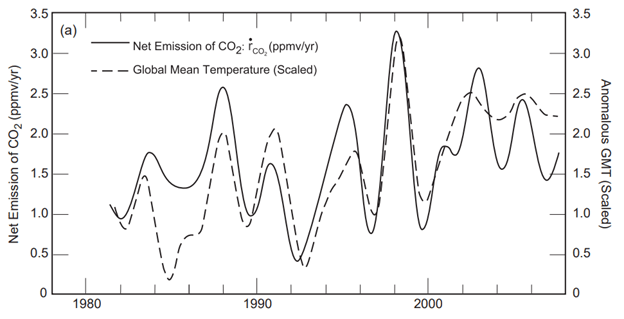
Meanwhile, net global average atmospheric CO₂ concentration is routinely and diligently measured in micromoles per mole (which is equal to parts per million or ppm) of atmosphere at Mauna Loa and a few other locations.  It has been observed by many scientists that net global average atmospheric CO₂ emissions vary with temperature.  In contrast, the common misunderstanding is that temperature varies with CO₂ concentration and global temperature is increasing because human-produced CO₂ is increasing.  While confirming that atmospheric CO₂ gas contributes to Earth’s temperature, atmospheric physicist, Professor Murry Salby, PhD has educated us that CO₂ varies coherently with temperature change, following temperature change, as shown in Figure 12. 

“An increase of T_S [surface temperature] introduced by a radiative perturbation dF [dF is the direct radiative forcing] thus leads to an increased emission rate of CO₂, and, hence, cumulatively in CO₂.” …”Increased temperature increases net emission of CO₂.  Decreased temperature has the reverse effect.  It is noteworthy that the positive sensitivity to temperature, dr_CO2/dT is not restricted to small perturbations. As is evident in Fig. 1.43, the dependence on temperature applies to r_CO2 as large as 100%.  Also noteworthy is that the correspondence applies to changes of temperature that are clearly of different origin.  Following the eruption of Pinatubo, when SW [shortwave radiation emitted by the sun] heating decreased, r_CO2 decreased by more than 50%. During the 1997-1998 El Nino, when SST increased, r_CO2 increased by more than 100%. To maintain stability, there must exist a negative feedback in CO₂, one that is sufficiently strong to bridle the enhancement of CO₂ emission by positive feedback from temperature.  That negative feedback involves sinks of CO₂ at Earth’s surface. (Salby, 2012).

As seen in the NOAA graph at the end of the introduction above, the time derivative of CO₂ concentration follows quickly in months the time derivative of sea surface temperature (SST). 

The link between sea surface temperature and CO₂ concentration also has been noted by government scientists.  For example: “At Mauna Loa the results implied that for the period 1970-1985, the season-to-season change would be about 0.2 ppm higher for a +1 degree C deviation in temperature of the eastern equatorial Pacific.  A slightly lower figured 0.15 ppm/degree C was found at the south pole for the full record length and about 0.35 ppm/degree C at Barrow (Alaska) for the full record.”…“For the cumulative dCO₂ we found a 1 degree C deviation would produce about 0.4 ppm change at Mauna Loa, 0.3 ppm change at the south pole, and 0.8 ppm at Barrow, Alaska.” (Elliott & Angell, 1986).

And “…we found as have others, that warming of this region is usually followed by an above average increase in CO₂ concentration.” …” At Mauna Loa this increase follows SST by about one season and at the south pole by two seasons.”  Unfortunately, these scientists usually do not pursue the linkage to its cause but instead, as these scientists did, the linkage or cause are dismissed. They concluded, “We take these results as further confirmation that the apparent effect of SST on the CO₂ record comes less from changes in the equatorial eastern Pacific than from climate changes throughout the globe.”  (Elliott et al., 1990).

Anthropogenic CO₂ is widely believed to be responsible for the trend of increasing net global average atmospheric CO₂ concentration, and from that belief it is inferred global temperature is increasing, some claim dangerously.  Proponents of anthropogenic CO₂-caused global warming (AGW) believe that reducing human CO₂ emissions by stopping the use of fossil fuels will reduce net global average atmospheric CO₂ concentration and thereby reduce global temperature.  The need to reduce global temperature is an unproven assumption as is the need to reduce human-produced CO₂.  Those assumptions are based on computer models where only a few types of data are measurements.  Comprehensive climate models have not been able to be validated against real world measured conditions.  For example, “The inability of current models to estimate accurately oceanic uptake of CO₂ creates one of the key uncertainties in predictions of atmospheric CO₂ increases and climate responses over the next 100 to 200 years. 60 references.” (Peng, 1987).

Climate scientists who support alleged human-caused global warming, for example Ben Santer and Michael Mann with others, authored a peer reviewed paper in the journal Nature Geoscience which acknowledges that their climate models are wrong, although their admission is hidden in technical jargon. They say in the first sentence of their paper’s abstract, “In the early twenty-first century, satellite-derived tropospheric warming trends were generally smaller than trends estimated from a large multi-model ensemble.” (Santer, 2017). In other words, the actual temperature trends were less than their modeled trends.  They continued, “Over most of the early twenty-first century, however, MODEL tropospheric warming is substantially larger than OBSERVED.” (Santer, 2017). (Capital letters are added for emphasis). In other words, their computer models substantially overestimate the global warming alleged to occur in the real world.

In contrast, the present study, based on measurements not models, simple in scope, analyzed a 2-year period where the rate of increase in slope of net global average atmospheric CO₂ concentration slowed and then stopped momentarily.  The acceleration of CO₂ concentration was temporarily halted by the effects of the Pinatubo volcanic eruption.  During those same months, CO₂ emissions from human sources continued, CO₂ emissions from natural sources continued (such as rotting soil and biosphere, etc.), the Pinatubo volcano itself added large amounts of CO₂ gas to the atmosphere, and an El Nino event in 1991-1992 added CO₂ to the atmosphere.  According to the results of this study, the second derivative (i.e., the acceleration) of CO₂ concentration dropped precipitously in the 2 years following Pinatubo to its lowest point in the pre-Pinatubo Mauna Loa record, despite the CO₂ additions by humans, natural sources, a volcano and an El Nino.  Nature rapidly absorbed the added CO₂ and then more rapidly accelerated again to reset its CO₂ concentration to trend.   

The Law of Mass Action states that the rate of a chemical reaction is directly proportional to the concentrations of the reactants, applicable under any circumstances.  In this case, the chemical reaction is the Henry’s Law phase-state equilibrium reaction of CO₂ occurring in millions of square kilometers of tropical seawater surface cooled by the effects of the Pinatubo eruption.  

To give the amounts of CO₂ perspective, Earth’s “…forests provide a “carbon sink” that absorbs a net 7.6 billion metric tonnes of CO₂ per year…” (World Resources Institute, 2021). Cooler surface in the two years following Pinatubo absorbed net 2778 billion metric tons of CO₂, and then in the next two years emitted that amount plus an additional increment.

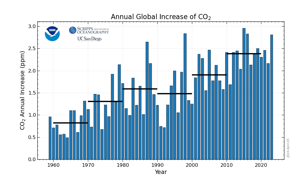
The rate of change of the slope of net global average atmospheric CO₂ concentration in this analysis dropped momentarily below zero. CO₂ concentration decelerated rapidly and briefly stopped growing. A large, global scale, decrease in CO₂ emission is consistent with an oceanic source of CO₂ and the rapid rate of change of slope is consistent with estimates of the size of absorption and emission fluxes of CO₂ gas from ocean and no where else.  By elimination, there is no other known, logical or physically possible sink for such a large amount of CO₂ to be absorbed so rapidly other than ocean surface.  The Henry’s global CO₂ dynamic equilibrium ratio was abruptly perturbed by cooling SST.  CO₂ emissions decreased precipitously after millions of square kilometers of tropical ocean surface cooled. Millions of square kilometers of ocean and land surface in higher latitudes also cooled. For a period of about 2 years, the rate of CO₂ absorptions into the environment greatly exceeded the rate of CO₂ emissions from all sources. The rate of change of CO₂ concentration (i.e., the slope of CO₂ concentration) had been on average 1.4 ppm per year since mid-1970s.  For a period of about 2 years, that slope decelerated and briefly reached below zero even though human emissions were continuing as usual, and the Pinatubo eruption had added large amounts of CO₂ to the atmosphere, and Earth’s biosphere was continuing to emit CO₂ as usual, and a El Nino event was adding CO₂ to the air.    

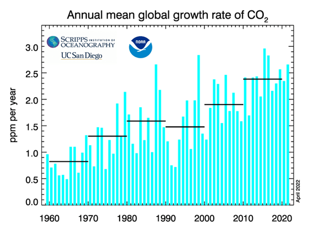
The decrease in CO₂ slope after 1991 followed by its recovery are clearly seen in the graph above.  This NOAA/Scripps graph is CO₂ slope versus time, i.e. ppm per year or velocity of net global average CO₂ atmospheric concentration.  1 ppm is 7.76 Gt of CO₂.    

Examining closely the NOAA/Scripps graph immediately above.  A slight decrease or flattening is visible after 1991.  This graph is CO₂ concentration versus time.   

In addition to the CO₂ added to the atmosphere by Pinatubo, and the continuing CO₂ emissions by humans from all sources, and the continuing natural emissions of CO₂ by the biosphere, there was an El Nino event in 1991-1992. El Nino events add large amounts of CO₂ to the atmosphere.  “The equatorial Pacific is the largest oceanic source of carbon dioxide to the atmosphere and has been proposed to be a major site of organic carbon export to the deep sea… The data establish El Nino events as the main source of interannual variability.” (Murray, 1994). The historical series of El Nino and La Nina perturbations are beyond the scope of this document, but we hope these major CO₂ and temperature perturbations can be examined in the next phases of this study.   

During the period 1990 to 1995, as mentioned, there were major additions of CO₂ to the atmosphere. We did not attempt to disentangle and quantify these additions. Yet our analysis revealed in MLO data a decrease in the slope of CO₂ concentration and a sharp temporary deceleration in CO₂ concentration. This begs the question: where did all of that CO₂ go? After about 2 years of deceleration, and a temporary halt in CO2 growth concurrent with ongoing human and large unusual but natural CO₂ additions, this rapid deceleration and halt was followed by an even more acceleration and recovery beyond the average rate of change of CO₂ concentration for the pre-Pinatubo decades.

Where did that CO₂ go?  Where did that recovery CO₂ come from?  It was and is in the ocean.  And it was there and is there in enormous quantity, as will be illustrated next. 

We studied the period of the Pinatubo perturbation.  A natural perturbation to the diligently measured approximate 20-year trend of CO₂ concentration occurred.  This Pinatubo perturbation period is an example, in both size and rates, of the capacity of the natural environment to emit and absorb CO₂.  Human-CO₂ emissions are also a perturbation to the same net global average CO₂ concentration trend, but tiny by comparison to Pinatubo’s perturbation.   

The CO₂ absorbed was over two orders of magnitude larger (over 100 times larger) than the perturbation due to human CO₂ emissions in the same period, as we will now show.  The rate of change (also known as slope, or velocity) of net global average CO₂ concentration averaged 1.463 ppm per year prior to Pinatubo.  After Pinatubo, the rate of change of concentration slowed. But the rate of change of the rate of change of CO₂ concentration declined very sharply. In other words, CO₂ slope decelerated to zero rate of change of slope. The growth of CO₂ concentration stopped and declined momentarily. By analogy, you did only ease off the gas pedal on the car after previously you were previously pushing down on the gas, accelerating to increase velocity, you took your foot off the gas and stepped down hard on the brake. Then, after reaching zero, for the next 2 years Earth accelerated rapidly, more rapidly than it had decelerated, to an average rate of change of concentration (i.e., average slope for the post Pinatubo period from 1995 to 2020) of 2.087 ppm per year. This remarkable recovery to trend with an offset above previous trend, that is an over recovery, is expected from Le Chatelier’s principle. The new slope after recovery is approximately a slope that would have been if the disturbance to trend had not occurred. This offset suggests that the CO₂ concentration has actual force and momentum, not only the statistical calculation of these physical concepts. This is pursued in the following analysis.

Rather than estimate natural and human emissions based on computer modeling, carbon budgets, proxy data from pre-industrial times, and dubious fossil fuel data sources, we will only compare CO₂ measured diligently by the Mauna Loa laboratory.   

On June 15, 1991, net global average CO₂ atmospheric concentration (Mauna Loa data) was 358 ppm. 

One ppm equals 7.76 gigatons (Gt) of CO₂.

358 ppm times 7.76 = 2778 Gt CO₂.

(1 ppm CO₂ = 2.12 Gt carbon. And 2.12 Gt carbon times 3.66 tonnes CO₂ per tonne carbon = 7.7592 Gt CO₂. Then 7.76 Gt CO₂ times 358 ppm CO₂ = 2778 Gt CO₂.)

The specific impulse calculation usually denoted J can be used to compare chemical forces in the environment. J is commonly used in chemistry, chemical engineering and health sciences to compare fluxes, that is, the mass of molecules moving in a vector direction through a surface area in a unit of time. For example, the directional flux of oxygen or anesthetic gas into lung tissue when inhaling.

Imagine a fully loaded 747 airplane with a mass of 2778 Gt on the runway ready to depart.  How did the jet engine and aircraft designers and later the pilots know that the engines could produce enough force to accelerate the airplane to sufficient velocity to become airborne before the end of the runway?  This calculation is the impulse calculation.  It gives us a reliable, well known and trusted calculation to compare human-produced CO₂ with natural CO₂.  If our 747 hits a bump in the runway and decelerates rapidly, then pilots or their computer must decide instantly: Can this plane take off before reaching the end of the runway? Does our 747 have enough force to accelerate to take-off velocity?  

The United Nations, leaders of over 100 nations through decades of government administrations in those nations, politicians and bureaucrats, judges, leaders of major industries, universities, mainstream media, the Pope in Rome, scientists and engineers who should know better, have been working vigorously for at least 40 years to convince you that the 747 must stop, turn around and go back to the gate. They have been telling us, attempting to scare us and scaring children worldwide, with practically non-stop, very expensive propaganda using our money, government policies and laws that the 747 will crash, that it does not have enough power to take off, that the 747 named Earth is in an existential crisis, life and death crisis, some alarmist claim the planet is beyond the point of no-return. They blame the trace gas CO₂ generated as a by-product of humans using fossil fuels.

We will now use the same calculation that pilots used thousands of times everyday to make life and death decisions, such as: can our airplane loaded with passengers, crew, baggage and fuel take off in time before reaching the end of the runway. This is known as the specific impulse calculation. The same physics and math used in the specific impulse calculation demonstrates that humans can not be responsible for global warming.  

This study provides the values measured by MLO for the critical variables in the specific impulse calculations for CO₂. The important variables are the same for both airplane and for CO₂ concentration. We have the mass of the airplane and the (measured, not estimated) mass of CO₂ in the air. And, we have the speed or velocity (or its rate of change of position) of the airplane, and we have the rate of change of CO₂ concentration in the air (aka the speed or velocity of the CO₂ concentration). And, we have the acceleration of the airplane (aka the rate of change of speed or velocity). And, we have the acceleration of the concentration of CO₂ in air (aka the rate of change of the velocity of CO₂ concentration). We will use these variables for the mass, velocity and acceleration of CO₂ concentration in atmosphere during the time period following the Pinatubo eruption to calculate the specific impulse of Earth’s environment. Does Earth’s environment have enough force to absorb human-produced CO₂ ? The mass of CO₂ is calculated from the MLO ppm concentration on the day of the Pinatubo main eruption.   

m = mass of net global average CO₂ concentration in air = 2778 Gt CO₂ in air, which is equal to 358 ppm CO₂ in air (measured by MLO June 15, 1991.) That is 2778 billion metric tons of CO₂.

dt is change in time = 2 years following Pinatubo eruption

a = acceleration

a = dv/dt   Acceleration a is the change in velocity divided by the change in time

a = 1.463 ppm/yr divided by 2 years = 0.73 ppm per year per year.

F is force.  F = m times a 

F = 2778 Gt CO₂ times 0.73 ppm/yr/yr = 2027.94 Newtons 

A Newton is the unit of force in the International System of units (SI).  It is represented by the symbol N. Sir Isaac Newton devised the three Laws of Motion.  The impulse-momentum theorem is logically equivalent to Newton’s second law of motion.  Impulse is the measure of force applied over time. Impulse is denominated by the symbol J.  J is always directional one-way (i.e. a vector).  The rate of change of molar concentrations and mass are compared in this illustration. There is no distance term, the mass is not moving over a distance in a unit of time as in the analogies of a car, airplane or rocket. But, our final comparison is a quotient, so the units drop out leaving a dimensionless ratio.

The physics term momentum M is perhaps more well known than specific impulse due to its use in sports. And we have the data to calculate M. M = force times velocity. Force is the mass of CO₂. Velocity is the slope of CO₂ concentration. M = F * v. Momentum is useful for atmospheric comparisons. But M does not tell us if the 747 can reach sufficient velocity to take off in a given time or runway. Similarly, M does not tell us if human CO₂ is increasing faster than the environment can remove it. For this comparison, we need specific impulse.

J = F times dt.   Impulse J = force times change in time

J = 2028 Newtons * 2 years

J =  4056  

4056 is the specific impulse of total CO₂ in the atmosphere on the day before the Pinatubo eruption.

For comparison, let’s assume human CO₂ was equal to 100% of the CO₂ that was added to the atmosphere between 1990 and 1991, the year preceding the Pinatubo eruption.  Calculating from MLO data, the measured average rate of change (or velocity) of net global atmospheric CO₂ concentration for year 1990 to 1991 was 1.463 ppm or about 1.5 ppm. How much CO₂ is that?  Thus 1.5 ppm times 7.76 Gt/ppm = 11.64 Gt of CO₂. 11.64 Gt is the total change in CO₂ concentration in the year 1990 to 1991; this amount exceeds maximum possible human emission in that year because it includes net CO₂ emissions from all sources and sinks of CO₂, not only human emission, all CO2 emitted from ocean, land, biosphere. But for the purpose of our comparison here, we will attribute 100% of that increase in CO₂ to humans.  Next, let’s also assume that 100% of the average velocity of human CO₂ emission continued during the 2 year period following the eruption even though the rate of total CO₂ was declining in that period. Our scientists calculated that average velocity in the pre-Pinatubo dataset period from 1970s to 1991 was 1.463 ppm/year.  Divide 1.463 by 2 years = 0.73.  

Repeating the specific impulse J calculation for maximum possible “human” CO₂:

F = mass times acceleration

J = F times dt.   Impulse J = force times change in time

11.64 Gt of “human” CO₂ times 0.73 ppm/year/year acceleration times 2 years = an impulse J of 16.99.

J is 17, the maximum possible specific impulse due to “human”-produced CO₂ that was added to the atmosphere during the 2-year post-Pinatubo deceleration period.  It is the maximum impulse because we assume (for the purpose of this comparison only) that all of the CO₂ increase from all sources since the 1970s is due to humans. 

The result of this comparison is exculpatory evidence.  We have J = 4056 for natural CO₂ removal in 2 years versus J = 17 for maximum possible “humans” addition of CO₂. The units drop out of the quotient leaving a dimensionless ratio 4056 / 17  = 239.

The environment, mostly ocean surface (since ocean is about 71% of Earth’s surface), demonstrated rapid CO₂ absorbance capacity which is 239 times larger than maximum possible amount of net human emissions.  We conclude that net human emissions are trivially minor, negligible, and absorbed and re-emitted along with the 239 times larger change in natural CO₂.  

Recall that deceleration of net global average CO₂ concentration dropped to near zero ppm/yr/yr.  CO₂ concentration, both natural and human, is cumulative over time.  Impulse is cumulative over time.  Thus, the impulse is suitable and logical for this comparative analysis.  Integration of cumulative CO₂ concentrations would also be a correct method for comparison, but the math is less well known.  Airliners would not be taking off without the impulse calculation.  Rockets would not reach orbit. When we attribute 100% of the changes in CO₂ concentration to humans, the impulse due to “humans” is negligible, not enough to stop CO₂’s rapid deceleration.  The human-produced-CO₂ climate change story does not fly. 

Conclusions:

The environment demonstrated a measured impulse to absorb 239 times the human-produced CO₂ impulse when very conservatively calculated.  Simply said, the natural environment is controlling CO₂ concentration. Human CO₂ emissions are not causing the increase in atmospheric CO₂.  The amount of human CO₂ emissions is negligible, less than a rounding error, in Earth’s specific impulse to absorb and emit CO₂ perturbations. And we do not yet know how large is Earth’s overall capacity; so far we have only calculated based on MLO measurements for the Pinatubo event. Henry’s Law, the Law of Mass Action and le Chatelier’s principle strongly suggest that net global average CO₂ concentration such as measured by MLO is controlled primarily by sea surface temperatures.  These temperatures are controlled by various natural forces.  Since an amount greatly exceeding all possible human CO₂ emissions was absorbed rapidly by the environment, then no net warming or net cooling can be attributed to human CO₂ emissions.  Our result suggests human CO₂ emissions are a minor perturbation which is rapidly returned to trend.       

Scientist P. Stallinga, PhD concluded, “The correlation between temperature and [CO₂] is readily explained by another phenomenon, called Henry’s Law: The capacity of liquids to hold gases in solution is depending on temperature. When oceans heat up, the capacity decreases and the oceans thus release CO₂ (and other gases) into the atmosphere. When we quantitatively analyze this phenomenon, we see that it perfectly fits the observations, without the need of any feedback [1]. We thus now have an alternative hypothesis for the explanation of the observations presented by Al Gore. The greenhouse effect can be as good as rejected and Henry’s Law stays firmly standing. We concluded that the effect of anthropogenic CO₂ on the climate is negligible and the effect of the ocean temperature on atmospheric [CO₂] is exactly, both sign and magnitude, equal to that as expected on basis of Henry’s Law.” (Stallinga, 2018, Stallinga, 2020).

Where did the CO₂ go after Pinatubo?  It was absorbed into the oceans primarily, and less into soils and the biosphere.  Our results strongly support the theory that the Henry’s Law dynamic equilibrium was adjusted downward due to the lower sea surface temperature, resulting in much less CO₂ being emitted from the cooled tropical ocean, soils and biosphere; meanwhile, normally colder water in higher latitudes was even colder due to the Pinatubo effects; net absorption increased in these higher latitudes.  Thus the CO₂ slope declined and acceleration rapidly declined post-Pinatubo.  Then, about 2 years after Pinatubo, when the cloud belt had partially dissipated and insolation of tropical oceans increased, then the deceleration of net global average atmospheric CO₂ concentration reversed sign and even more rapidly recovered. Average slope following the recovery was a step higher than the pre-Pinatubo average. Professor Murry Salby provides calculations and graphs showing that the observed long-term slope of CO₂ concentration is explained by a series of offsets such as Pinatubo and El Ninos. “There is no evidence of a systematic trend in temperature.” [referring to the actual mean global University of Alabama Huntsville’s satellite records for global anomalous temperature.] (Salby, 2018, beginning about 16:30 time mark in the video).

Concerning the Pinatubo perturbation, Stallinga and Khmelinskii (2018) write, “In total, the natural contribution is negative 50% of the anthropogenic emissions (i.e., a sink; Sabine, C.L. et al. estimate 48% ( Sabine, C.L. et al., 2014), plus fluctuations, with these fluctuations being of the same order of magnitude as the anthropogenic emissions… We have thus direct proof of Henry’s Law that predicts such effects of temperature on the carbon-dioxide content in the atmosphere. Oceans undeniably outgas and absorb CO₂ from the atmosphere and they govern the dynamics, the correlation of [CO₂] with temperature.” (Stallinga & Khmelinskii, 2018).   In other words, human emissions are absorbed by nature. 

Kauppinen and Malmi (2019) explain, “Low cloud cover controls practically the global temperature.” “The IPCC climate sensitivity is about one order of magnitude too high, because a strong negative feedback of the clouds is missing in climate models. If we pay attention to the fact that only a small part of the increased CO₂ concentration is anthropogenic, we have to recognize that the anthropogenic climate change does not exist in practice. The major part of the extra CO₂ is emitted from oceans [6], according to Henry‘s law. The low clouds practically control the global average temperature. During the last hundred years the temperature is increased about 0.1°C because of CO₂. The human contribution was about 0.01°C.” (Kauppinen & Malmi, 2019).

Since the Pinatubo cloud belt around Earth’s equator mostly obfuscated insolation of normally warm tropical ocean surface, and since CO₂ gas solubility in sea surface is inversely proportion to SST, we confidently deduce that the measured, rapid deceleration of CO₂ concentration was caused by cooling of millions of square kilometers of tropical ocean surface.  Our result and the novel use of the standard specific impulse calculation reveal a MLO-measured net CO₂ gas absorption impulse more than 230 times larger than the MLO-measured maximum possible net human emission impulse during the same time period.  We expect that continuing this study into its next phases will yield a matrix of supporting evidence and, possibly, a calibration curve for human-CO₂ emissions, based on measurements rather than estimates, so that the pernicious claims of global climate change due to human-produced CO₂ can be summarily dismissed.  The argument that human-CO₂ emission is causing global climate change is shown to have no scientific merit. 

Credits and Acknowledgements

Thoning et al (2021). K.W. Thoning, A.M. Crotwell, and J.W. Mund (2021), Atmospheric Carbon Dioxide Dry Air Mole Fractions from continuous measurements at Mauna Loa, Hawaii, Barrow, Alaska, American Samoa and South Pole. 1973-2020, Version 2021-08-09 National Oceanic and Atmospheric Administration (NOAA), Global Monitoring Laboratory (GML), Boulder, Colorado, USA https://doi.org/10.15138/yaf1-bk21

FTP path: ftp://aftp.cmdl.noaa.gov/data/greenhouse_gases/co2/in-situ/surface/

The software toolset for this initial phase of the study was designed and operated by Shahar Ben-Menahem, PhD (physics, Stanford) and Abraham Ishihara, PhD (Aeronautics & Astronautics, Stanford) through their company Modoc Analytics LLC. 

This study, referred to by the scientific team, management, and ClimateCite Corporation as the “Pinatubo Study – phase I”, was entirely funded by Tomer Tamarkin, Carmichael, CA with the generous help and support of Pat Boone, Beverly Hills, CA.  No financial solicitations were made to any other corporations, companies, or individuals, nor funds received.  Intellectual work product and copyright, 2022, ClimateCite Corp.

Bud Bromley has no conflicts of interests which might affect the direction of this study or authoring this report. This report is also available here: https://budbromley.blog/2022/05/20/correcting-misinformation-on-atmospheric-carbon-dioxide/  

Glossary

An extensive glossary of names, terms, & scientific principles used in this paper may be found online at: https://pinatubostudy.com/glossary.html

References

Cohen, R., & Happer, W., (2021, November 21). Fundamentals of Ocean pH. CO2 Coalition.org. https://co2coalition.org/publications/fundamentals-of-ocean-ph/

Elliott, W.P., & Angell, J.K., (1987). On the relation between atmospheric C02 and equatorial sea-surface temperature. Tellus B: Chemical and Physical Meteorology, 39B, 171-183.  https://www.tandfonline.com/doi/pdf/10.3402/tellusb.v39i1-2.15335

Elliott, W.P., Angell, J.K., & Thoning, K.W. (1990). Relation of atmospheric CO2 to tropical sea and air
temperatures and precipitation. Tellus 43B: Chemical and Physical Meteorology, 43:2, 144-155, : https://doi.org/10.3402/tellusb.v43i2.15259

Friedlingstein, P., Jones, M. W., O’Sullivan, M., Andrew, R. M., Bakker, D. C. E., Hauck, J., Le Quéré, C., Peters, G. P., Peters, W., Pongratz, J., Sitch, S., Canadell, J. G., Ciais, P., Jackson, R. B., Alin, S. R., Anthoni, P., Bates, N. R., Becker, M., & Bellouin, N., (2021) Global Carbon Budget 2021, Earth Syst. Sci. Data Discuss. [preprint], https://doi.org/10.5194/essd-2021-386

Harde, H. (2019).  What Humans Contribute to Atmospheric CO2: Comparison of Carbon Cycle Models with Observations. Earth Sciences. Vol. 8, No. 3, 2019, pp. 139-158. https://doi.org/doi: 10.11648/j.earth.20190803.13

Henry, W. (1803). Experiments on the quantity of gases absorbed by water, at different temperatures, and under different pressures. Phil. Trans. R. Soc. Lond. 93: 29–274. https://doi.org/doi:10.1098/rstl.1803.0004

Hoppe, K. (1992).  Mt. Pinatubo’s cloud shades global climate. Science News. July 18, 1992. https://www.thefreelibrary.com/Mt.+Pinatubo’s+cloud+shades+global+climate.-a012467057

Kauppinen, J., & Malmi, P. (2019). No experimental evidence for the significant anthropogenic climate change.  Cornell University. arXiv:1907.00165v1 [physics.gen-ph] 29 Jun 2019. https://arxiv.org/abs/1907.00165v1

Mauna Loa Observatory, 2005. USGov-Doc. http://www.cmdl.noaa.gov/albums/cmdl_overview/Slide18.sized.png. https://en.wikipedia.org/wiki/File:Mauna_Loa_atmospheric_transmission.png

Mazza, D. (accessed 2022, April 15) Academia.edu   https://danielemazza.academia.edu/

Mazza, D. (2020). Algorithms in Ocean Chemistry. ISBN | 978-88-31688-62-8.  https://www.academia.edu/attachments/64182996/download_file?s=portfolio

Murray J.W., Barber R.T., Roman, M.R., Bacon, M.P., & Feely, R.A. (1994) Physical and biological controls on carbon cycling in the equatorial pacific. Science. 1994 October 7;266(5182):58-65. https://www.science.org/doi/10.1126/science.266.5182.58

Onuki, Akira (2009). Henry’s Law, surface tension, and surface adsorption in dilute binary mixtures. J. Chem. Phys. 130, 124703.  https://doi.org/10.1063/1.3089709
https://doi.org/10.48550/arXiv.0902.1204

Peng, T-H, Post, W. M., DeAngelis, D. L., Dale, V. H., & Farrell, M. P. (1987) Atmospheric carbon dioxide and the global carbon cycle: The key uncertainties. United States. https://www.osti.gov/biblio/5473519-atmospheric-carbon-dioxide-global-carbon-cycle-key-uncertainties

Sabine, C.L., Feely, R.A., Gruber, N., Key, R.M., Lee, K., Bullister, J.L., Wanninkhof, R., Wong, C.S., Wallace, D.W.R., Tilbrook, B., Millero, F.J., Peng T-H, Kozyr, A., Ono, T., & Rios, A.F. (2004) The Oceanic Sink for Anthropogenic CO2. Science, 305, 367.
https://doi.org/10.1126/science.1097403

Salby, M.L. (2012). Physics of the Atmosphere and Climate. 2nd Edition. ISBN: 9780521767187. https://climatecite.com/physics-of-the-atmosphere-and-climate-pt-1/  and https://climatecite.com/physics-of-the-atmosphere-and-climate-pt-2/

Salby, M.L., & Helmut-Schmidt-University Hamburg. (2018, October 10). What is Really Behind the Increase of Atmospheric CO₂ ? [Video]. YouTube. https://youtu.be/rohF6K₂avtY

Sander, R. (2015). Compilation of Henry’s law constants (version 4.0) for water as solvent. Atmos. Chem. Phys., 15, 4399–4981, 2015. https://doi.org/10.5194/acp-15-4399-2015 and https://henry.mpch-mainz.gwdg.de/henry/

Santer, B.D., Fyfe, J.C., Pallotta, G., Flato, G.M., Meehl, G.A., England, M.H., Hawkins, E., Mann, M.E., Painter, J.F., Bonfils, C., Cvijanovic, I., Mears, C., Wentz, F.J., Po-Chedley, S., Fu, Q., & Zou, C-Z. 2017. Causes of differences in model and satellite tropospheric warming rates. Nature Geoscience. 19 June 2017. http://www.meteo.psu.edu/holocene/public_html/Mann/articles/articles/SanterEtAlNatureGeosci17.pdf

Stallinga, P. (2018). Carbon dioxide and ocean acidification. European Scientific Journal June 2018 edition Vol.14, No.18. https://doi.org/10.19044/esj. http://dx.doi.org/10.19044/esj.2018.v14n18p476

Stallinga, P. (2018). Signal analysis of the climate: correlation, delay and feedback. Journal of Data Analysis and Information Processing, 6, 30-45. https://doi.org/10.4236/jdaip.2018.62003

Stallinga, P. (2020). Comprehensive analytical study of the greenhouse effect of the atmosphere. Atmospheric and Climate Sciences, 10, 40-80. https://doi.org/10.4236/acs.2020.101003

Stallinga, P., & Khmelinskii, I. (2018). Analysis of temporal signals of climate, Natural Science, Vol.10 No.10, 2018. https://doi.org/10.4236/ns.2018.1010037

Stenchikov, G., Ukhov, A., Osipov, S., Ahmadov, R., Grell, G., Cady-Pereira, K., Mlawer, Mlawer, E., & Iacono, M. (2021).  How does a Pinatubo-size volcanic cloud reach the middle stratosphere? JGR Atmospheres. 14 May 2021.  https://doi.org/10.1029/2020JD033829

Stumm, W., & Morgan, J.J. (1996).  Aquatic Chemistry: chemical equilibria and rates in natural waters.  James J. Wiley Interscience.192. https://archive.org/details/aquaticchemistry0000stum/mode/2up

Tans, P.P. (2006). Acceleration of the rate of growth of atmospheric carbon dioxide. NOAA Earth System Research Laboratory. https://gml.noaa.gov/publications/annual_meetings/2006/abstracts/talks_2006_02.pdf

The Engineering Toolbox. (accessed 2022, April 15) The Solubility of Gases in Water vs Temperature. The Engineering Toolbox.  https://www.engineeringtoolbox.com/gases-solubility-water-d_1148.html

Thoning, K.W., Crotwell, A.M., & Mund, J.W. (2021). Atmospheric carbon dioxide dry air mole fractions from continuous measurements at Mauna Loa, Hawaii, Barrow, Alaska, American Samoa and South Pole. 1973-2020, Version 2021-08-09. National Oceanic and Atmospheric Administration (NOAA), Global Monitoring Laboratory (GML), Boulder, Colorado, USA https://doi.org/10.15138/yaf1-bk21 Data Set Name: co2_mlo_surface-insitu_1_ccgg_DailyData. Description: Atmospheric carbon dioxide dry air mole fractions from quasi-continuous measurements at Mauna Loa, Hawaii.

Harris, N., & Gibbs, D. (2021, January 21). Forests absorb twice as much carbon as they emit each year.  World Resources Institute. https://www.wri.org/insights/forests-absorb-twice-much-carbon-they-emit-each-year

Zeebe, R.E., & Wolf-Gladrow, D.A. Carbon dioxide, dissolved (ocean). University of Hawai’i at Manoa. https://www.soest.hawaii.edu/oceanography/faculty/zeebe_files/Publications/ZeebeWolfEnclp07.pdf

#ClimateChange #IPCC #GlobalWarming #ClimateCrisis #Sustainability #NetZero #EPA #EndangermentFinding #CO2 #ClimatePolicy #EnergyPolicy #FossilFuel #Henry’sLaw