
The error in Friedlingstein et al (2021) is much larger than expected. Friedlingstein et al Page 4: “total anthropogenic CO2 emission of 10.2 ± 0.8 GtC yr-1 (37.4 ± 2.9 GtCO2).”
The amounts above are their calculation, not mine.
Friedlingstein et al reported their estimate for 1 year’s (2020) increase for human fossil fuel emissions, land use and cement = 37.4 +- 2.9 Gt CO2. This is their estimate of emissions not net emissions. Net CO2 absorption has not been subtracted.
Follow this simple arithmetic:
• Using NOAA Mauna Loa data only (no estimates, no theories, no models, no assumptions.) Reported in micromoles/mole = ppm.
• MLO did not report CO2 flask measurements on Jan 1, 2020
• 2 Jan 2020, MLO reported 4 CO2 flask measurements for Jan 2, 2020. Average 412.9875 ppm
• 31 Dec 2020, MLO reported 4 CO2 flask measurement for Dec 31, 2020. Average 415.5225 ppm
• CO2 increase due to all sources human and natural combined for year 2020 is 2.535 ppm, (i.e., 415.5 minus 412.9875)
• 2.535 ppm CO2 per year times 7.76 Gt CO2 per ppm of CO2 = 19.679 Gt CO2 added to the atmosphere in 2020 from all sources human and natural.
• Thus, net CO2 added by humans cannot exceed 19.679 Gt CO2 in 2020, because this amount includes net CO2 additions by all sources.
• Net global average CO2 concentration reported by Mauna Loa on 31 December 2020, the average of 4 measurements that day was 415.5225 ppm. Multiply by 7.76 Gt per ppm = 3224.455 Gt CO2 total CO2 in atmosphere.
• Then, 19.679 / 3224.455 = 0.006103. Multiply by 100 = 0.610%.
• Net Human CO2 added to air in 2020 cannot exceed 0.610% of total CO2 for 2020. This 0.61% includes net CO2 emissions and net CO2 absorptions from humans including cement, net CO2 from ocean, net CO2 from land, rivers, lakes, CO2 from rotting and decay, net CO2 from biosphere, etc.
37.4 Gt CO2 is the Friedlingstein et al estimate of human emissions only for 2020. It is an excessively complicated estimate. If you read the Friedlingstein et al paper you will see the complications, uncertainties, and assumptions. But that amount is human emissions only and only emissions, that is CO2 absorptions have not been subtracted from their estimated human CO2 emissions.
Net total CO2 added in 2020 was measured 19.679 Gt CO2. 37.4/19.7 = 52.7%, but this is an apples and oranges comparison. 19.7 is total emissions minus total absorption. 37.4 is human only and emissions only. Friedlingstein et al has a major problem. We do not know how much of that 37.4 Gt CO2 human emission was absorbed during 2020. But we do know that net human emissions cannot exceed 19.679 Gt CO2.
It is easily proven and observed that ocean is both a CO2 sink and a CO2 source. CO2 flux is non-stop in both directions, into and out of Earth’s surface. Earth’s surface is over 70% ocean. CO2 gas molecules continuously collide with ocean surface, day and night, regardless of season, temperature, or location; some of that CO2 is emitted back into air, and some is retained in the surface. The partition ratio of CO2 between gas in the surface versus gas above the surface is the Henry’s Law coefficient. The coefficient is a simple ratio of CO2 moles or mass; it varies with the local surface temperature. The resulting ratio is a dimensionless, intensive property of matter. Adding more CO2 to the air or to the ocean surface does not change the CO2 ratio. Diffusivity of a gas in a liquid is a function of the mass of the gas, specifically the inverse of the square root of the molecular weight of the gas. Humans, volcanoes, biosphere, etc., adding CO2 to the atmosphere does not change the Henry’s ratio or diffusivity of the CO2 gas into the ocean surface. The concentration of CO2 gas in the ocean surface and in the air at a given local surface temperature is given by the Henry’s Law coefficient plus or minus temporary perturbations due to alkalinity, surface or air disturbances due to winds, currents, and salinity at that location. The net amount of biosphere CO2 flux, another perturbation, is also non-stop in both directions when CO2 emissions due to decay are included. These perturbations adjust by CO2 emission or CO2 absorption and rapidly return to the Henry’s Law CO2 partition ratio.
Friedlingstein et al say on Page 9: “Global emissions and their partitioning among the atmosphere, ocean and land are in reality in balance.”
Friedlingstein et al calculate on page 32, section 3.4.2, “The observed stability of the airborne fraction over the 1960-2020 period indicates that the ocean and land CO2 sinks have been removing on average about 55% of the anthropogenic emissions (see sections 3.5 and 3.6).”
Apparently, Friedlingstein et al believe nature is in balance, except for humans. Apparently, they believe that nature, which balances 3224.455 Gt CO2 total CO2 in atmosphere by continuous emissions and absorptions, is unable to balance an additional estimated 37.4 Gt CO2 from humans. Nature is already balancing over 86 times more CO2 than their estimation of human emissions, (i.e., 3224.5/37.4) but for some unexplained reason they believe nature is unable to balance the relatively tiny human CO2 perturbation, a human amount which is much less than 0.61% of the total, (i.e., 19.7/3224.5) because that 0.61% includes net CO2 emissions from all sources and sinks, human and natural.
Even the above example understates the size of their error. Since net human emissions would be a cumulative net of two fluxes, if there were a method to measure it, and since net global average CO2 concentration (i.e., NOAA Mauna Loa) is the net of two giant CO2 fluxes in opposite vector directions, then we should compare these data as integral areas. (That is still an apples and oranges comparison because we only have the estimate of human emissions, not net human emissions. But at least the comparison would be in the right order of magnitude.)
Follow this simple arithmetic:
- Friedlingstein et al estimate 37.4 Gt human CO2 emissions for 2020. For avoidance of doubt, this is not emission minus absorption.)
- 1 ppm CO2 equals 7.76 Gt CO2
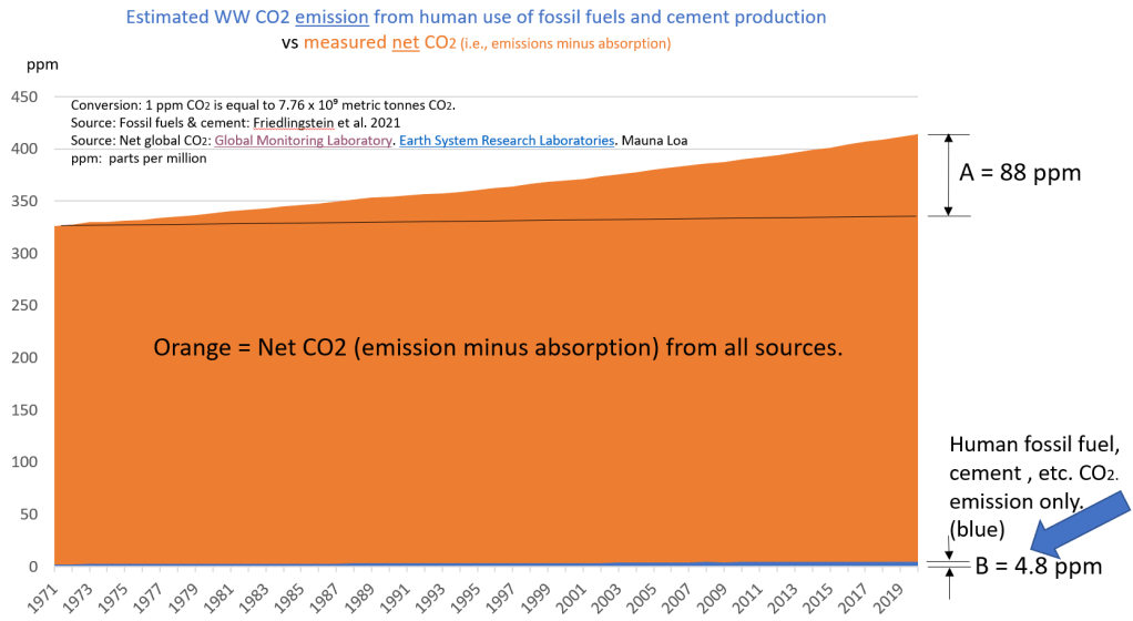
- 37.4 Gt divided by 7.76 = 4.8195 ppm human CO2 emissions for 2020, call it 4.8 ppm
Then the comparison between total CO2 versus Friedlingstein et al estimated human CO2 emission would look something like the following graphic. We compare the entire area of the orange quadrangle to the area of the thin blue quadrangle. Absorptions of human CO2 emissions have not been subtracted. Nevertheless, it should be obvious that B is not causing A, and the orange area is enormously larger than the blue area.
Human emissions cannot be driving the growth rate (slope) observed in net global average CO2 concentration.
Net global average CO2 concentration in air today is the same as it would be if humans never existed.
References
- Friedlingstein et al. (2021) https://essd.copernicus.org/preprints/essd-2021-386/essd-2021-386.pdf
- K.W. Thoning, A.M. Crotwell, and J.W. Mund (2022), Atmospheric Carbon Dioxide Dry Air Mole Fractions from continuous measurements at Mauna Loa, Hawaii, Barrow, Alaska, American Samoa and South Pole. 1973-2021, Version 2022-05 National Oceanic and Atmospheric Administration (NOAA), Global Monitoring Laboratory (GML), Boulder, Colorado, USA. https://doi.org/10.15138/yaf1-bk21
- Dlugokencky, E.J., J.W. Mund, A.M. Crotwell, M.J. Crotwell, and K.W. Thoning (2021), Atmospheric Carbon Dioxide Dry Air Mole Fractions from the NOAA GML Carbon Cycle Cooperative Global Air Sampling Network, 1968-2020, Version: 2021-07-30, https://doi.org/10.15138/wkgj-f215 download file here: https://budbromley.blog/wp-content/uploads/2022/11/raw-unparsed-daily-esrl-mlo-1973-to-2020-2.xlsx
- Bromley, B., & Tamarkin, T. (2022). Correcting misinformation on atmospheric carbon dioxide. https://budbromley.blog/2022/05/20/correcting-misinformation-on-atmospheric-carbon-dioxide/
#ClimateChange #IPCC #GlobalWarming #ClimateCrisis #Sustainability #NetZero #EPA #EndangermentFinding #CO2 #ClimatePolicy #EnergyPolicy #FossilFuel #Henry’sLaw

Pingback: In Defence of Non-IPCC CO2 Science | Science Matters
Pingback: By the Numbers: CO2 Mostly Natural | Science Matters
Bud, thanks for your work on this paper. Honestly, I haven’t deep knowledge of IPCC carbon budgeting methods, and this paper gets into the complexities of it. I struggle to get to the core of the matter, in order to explain it in simple terms. My concerns are that the two very different CO2 fluxes are not handled transparently. Fossil Fuel emissions are a simple addition (one way) while natural sources and sink are two way, and must be integrated over time. Furthermore, there is the matter of large error ranges in all of the estimates, such that FF emissions are smaller than the cumulative error ranges. A summary:
Several things are notable about the carbon cycle diagram from GCP. It claims the atmosphere adds 18 GtCO2 per year and drives Global Warming. Yet estimates of emissions from burning fossil fuels and from land use combined range from 36 to 45 GtCO2 per year, or +/- 4.5. The uptake by the biosphere and ocean combined range from 16 to 25 GtCO2 per year, also +/- 4.5. The uncertainty on emissions is 11% while the natural sequestration uncertainty is 22%, twice as much.
Furthermore, the fluxes from biosphere and ocean are both presented as balanced with no error range. The diagram assumes the natural sinks/sources are not in balance, but are taking more CO2 than they release. IPCC reported: Gross fluxes generally have uncertainties of more than +/- 20%. (IPCC AR4WG1 Figure 7.3.) Thus for land and ocean the estimates range as follows:
Land: 440, with uncertainty between 352 and 528, a range of 176
Ocean: 330, with uncertainty between 264 and 396, a range of 132
Nature: 770, with uncertainty between 616 and 924, a range of 308
So the natural flux uncertainty is 7.5 times the estimated human emissions of 41 GtCO2 per year.
LikeLike
Thanks for reading and commenting Ron. I fixed the typo MKO which should be MLO, an abbreviation for the Mauna Loa Laboratory of the Global Monitoring Laboratory of jointly run by NOAA and Scripps Oceanographic Institute.
As you probably know, MLO is the gold standard measurement of the net global average atmospheric CO2 concentration.
Carbon budgeting is a computer game. The purpose of the computer game is to keep the computer game going. We can talk about that separately if you wish, but I won’t comment further in this message except to say that your digging will take you nowhere, and they know that. The simultaneous partial differential equations cannot be solved (even with the largest and fastest supercomputers) with scientifically acceptable levels of uncertainty.
Regarding your question about 2020 CO2. Well, this is fundamental to understanding what is really happening. Nothing special about 2020. It just happens to be the most recent carbon budget published by these 60 or so computer gamers who call themselves climate scientists. The 2020 data is in their 2021 carbon budget report, and this is apparently still a pre-print subject to change. There is also nothing special about the 2020 CO2 data, I could do the same calculation for 2021 or 2019, 1991, etc.
1: My calculations are using only measured data for CO2. That is, no estimates, no assumptions, no computer models.
2: I use in this post only arithmetic, so that anyone who reads the post can understand if they make the effort. Integral calculus would also be correct, and some statistics are correct, but most people do not understand those methods.
3. The net CO2 increase due to all sources human and natural for year 2020 was 2.5350 ppm. This converts to Gt CO2 by multiply by 7.76 GtCO2 per ppm of CO2 in air. The result is 19.679 Gt CO2 added to the atmosphere in 2020 from all sources human and natural.
4. This means that for the year 2020, human CO2 emissions minus of all absorptions of those CO2 emissions cannot exceed 19.678 Gt CO2. Do you follow this so far?
5. Net global average CO2 atmospheric concentration reported by MLO on 31 January 2020 was 415.5225 ppm. Multiply by 7.76 Gt per ppm = 3224.455 Gt CO2 total CO2 in atmosphere. This is the net of all sources human and natural. And this is the net residual difference between two gigantic CO2 fluxes, the net emission flux from all sources from ocean surface into air, versus the net absorption flux from air into all CO2 sinks. Absorption and emission are both continuous processes. CO2 gas is always colliding with the surface. Do you follow this so far?
6. Divide 3224.455 GtCO2 (from #5 above) by 19.678 Gt CO2 (from #4 above) gives us 0.006103. Multiply that by 100 gives us 0.61%. Therefore, net human CO2 emissions cannot exceed 0.6% of net global average CO2 concentration for 2020. Do you follow this?
7. There is no so-called “airborne fraction” of human CO2. All human CO2 added to the atmosphere in 2020 is included in the above arithmetic and measurements.
Note there is no averaging in my calculation in the sense of an annual average or global CO2 average as done by an arithmetic mean of a large same population of data points. The net global average CO2 concentration data mentioned here is an averaging done by nature, as in CO2 gas measured by MLO is assumed to be “well mixed” by natural environmental processes. It is not a arithmetic operation. It assumes CO2 gas is well mixed in air and that MLO is taking a sample that represents the global average. I averaged 4 discrete, MLO-measured data points on January 2, 2020. Separately, I averaged 4 discrete MLO-measured data points for Jan 31, 2020. Averaging of averages is a major problem in climatology literature. I have not averaged any averages.
8. Now if we go back to any previous point in time when there is a MLO measurement, we can use the exact calculation as above to calculate annual increase in CO2 during that year, and we can calculate the net CO2 concentration for that year. I went back to the earliest MLO discrete flask measurements and found MLO net CO2 was 327 ppm. Jan 31, 2020 was 415.5225 ppm. 415 ppm minus 327 = 88 ppm. This is “A” in my simple graphic. So, 88 ppm is net total increase in CO2, the net of all emissions minus the net of all absorptions from all sources human and natural during that multi-decade time.
9. The human CO2 increase (as calculated above) cannot exceed 0.61% of the net global average CO2 concentration on Jan 31, 2020. Then 0.61% X 415.5225 ppm = 2.53 ppm maximum possible net human emissions. This is an extremely conservative “not to exceed” amount because it includes all CO2 from all sources. In the graphic in my blog post I used 4.8 ppm since this was the amount calculated by Friedlingstein et al for human emissions. This Friedlingstein et al is an estimate, not a measurement. And it is human emissions only; they do not know what part of that 4.8 ppm is absorbed. This is their “atmospheric fraction” computer game of circular logic beginning from a dubious estimate. On the other hand, 2.53 ppm is a MLO-measured amount which includes the net of all human and all natural absorptions and emissions; this is a known cumulative amount of increase at Jan 31, 2020. In other words, 2.53 ppm is an accurate measurement, but 4.8 ppm is an uncertain guess.
10. There are many comparisons that can be made. One is to divide 2.53 ppm (from #9 above) by 88 ppm (from #8 above) = 39.5%. This tells us that net human emissions are only 39.5% of the measured INCREASE in net global atmospheric CO2 concentration since 1971. That begs the obvious question, where did the 60.5% of CO2 come from. That is a question I hope to answer in a future post. Our result from Bromley and Tamarkin (2020) suggests the incremental CO2 came from ocean surface.
11. #1 through #10 already shows that the amount of human CO2 is trivial and negligible. This means addition of human CO2 from fossil fuels causes no harm to the environment, and removal of human CO2 from fossil fuels produces no benefit to the environment.
12. Now there are further ways to disprove Friedlingstein et al, IPCC, world bankers and governments, etc. (Not that I expect that they are reading or care. They ignore and disparage far more famous and credited scientists for years. They won’t give up their computer games until their funding is taken away. This argument is not about veracity, science or justice.) But, if you want further proof and comparisons, then you could integrate the orange quadrangle and compare it to the integral of the thin blue quadrangle for the years in the graphic or for any other years you wish. (Do not use averages or estimates.) Another comparison would be to pick a year and analyze the variance and standard deviation within year for MLO daily measurements. (Don’t use MLO annual data or monthly data because these data use averages.) Keeping in mind that the MLO data is the net residual difference between two much larger CO2 fluxes, you will find that the variance and standard deviation in the daily MLO data is much larger than the maximum possible human CO2 addition for the same period. In other words, there is a signal-to-noise problem and it is ignored. This is the reason to compare the data as in #1 through #1 or in my blog posts. Advanced signal analysis may be able to disentangle the signal of human CO2 from total CO2. We will see about that.
13. Another comparison is to demonstrate by chemistry and calculations that ocean surface emits and absorbs fluxes of CO2 that are orders of magnitude more CO2 than maximum possible human CO2 net emission flux. I have started these calculations.
Ron, or anyone reading this, let me know if you have questions.
LikeLike
Bud, some confusion (typos?) in your post which I don’t get. MKO? I suppose should be MLO. Why a one month period Jan. 2, 2020 to Jan 31, 2020?
LikeLike
Bud
Could you look at the attached note I have put together re emissions v atmospheric CO2
Does it make sense?
LikeLiked by 1 person
I do not see a note attached. Please send by email. I will be happy to review.
LikeLike
I do not see your note. Please send to bud.bromley@outlook.com
LikeLike
Bud
There is so much obfuscation
IPCC use the fact that annual emissions are on average half the annual atmospheric increase, to âproveâ that half of emissions are sequestrated by the biosphere and oceans, but they conveniently ignore the fact that emissions are around 4.2% of the 100ppm annual flux of global absorption & desorption.
Yes the average difference between emissions and atmospheric ppm since 1965 is 50%, but each year emissions can be as little as 14% or as much as 80% of atmospheric value, beware averages, the average human has 1 breast and 1 testicle?
The graph below is Gt CO2 fossil fuel (blue) and Total (grey) and annual increase in atmospheric CO2 (Orange).
Emissions rise and fall monotonically, sometimes falling below the previous year, atmospheric is always more than the previous year, and must be driven by something else (SSTs)?
Neither the grey nor blue curves, which are deviating away from the atmospheric trend, can be âdrivingâ the atmospheric/orange curve?
Best wishes
Howard
[cid:image001.jpg@01D88ED8.E69D7AB0]
LikeLike
Howard, I am unable to open the graph. Can you send it by email?
Which emissions are “around 4.2% of the 100ppm annual flux of global absorption & desorption.”?
Yes, indeed averages are not good. The only average I used are the two averages of the 4 flask samples within Jan 2, 2020 and Jan 31 2020. That is no problem. But the Freidlingstein papers are loaded with averages and estimates. Obfuscation. In the analytical instrumentation business, this was one of the sources of data closure. One degree of freedom is lost for each average of an average. This is a big but largely unrecognized problem with the pervasive use of anomalies in climate literature. The practice reduces the standard deviation in the data, resulting in overconfidence in the result.
By itself, the human emissions number is dubious because over the years some of the largest fossil fuel suppliers have “managed” their fossil fuel production data for political and business reasons, including Soviet Union, OPEC, Iran, Venezuela and Nigeria. But, worse yet, then IPCC and Friedlingstein et al and their followers use that dubious number to calculate a carbon balance when they can only guess at the amount of absorption of those emissions. That is circular logic beginning from a dubious starting point. Like a plug in a spreadsheet when the data does not “foot” or tally correctly. They use 50% because that’s the number that makes their calculation look right for propaganda purposes. What I show here in this blog post is that it cannot be 50% (or anywhere close to 50%) because the measured net of all emissions from all sources human and natural minus the net of all absorptions from all sources human and natural (i.e., the measured annual change in Mauna Loa concentration for 2020) is only 0.61% of the measured net global CO2 concentration from all sources human and natural. No algebra, calculus, estimates, averages, assumptions or computer models, only arithmetic.
Then simply looking at difference between the area of orange quadrangle versus the area of the blue triangle, human emissions will be a tiny, tiny fraction of 0.61% of the total CO2.
LikeLike
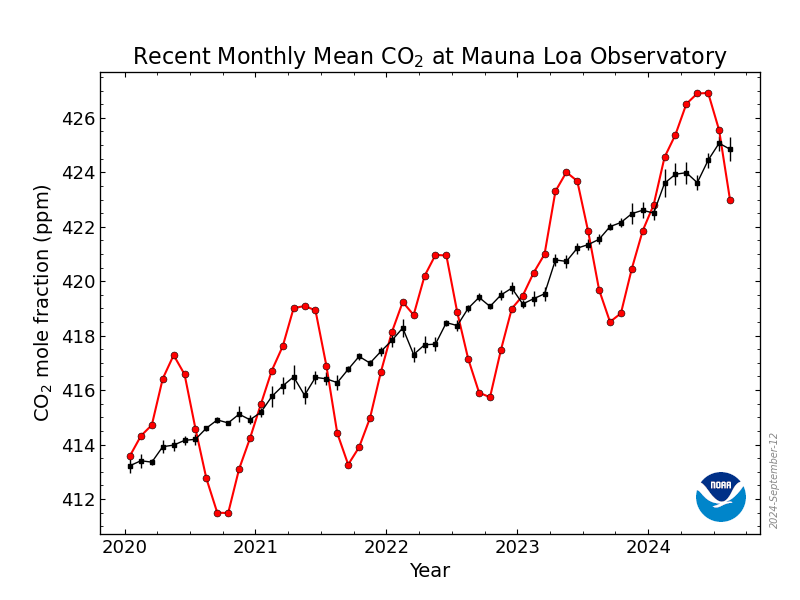
If further evidence of the lack of anthropogenic signal in the atmospheric CO 2 concentration, the absolute lack of any perturbation of the Mauna Loa CO2 graph by the (estimated) 10% reduction in anthropogenic emissions should do rather nicely.
LikeLike
Yes, the failure to see a response in CO2 record due to the reduction of fossil fuel emissions during the near-global covid shutdowns points to the statistical insignificance of fossil fuel emissions. Human emissions are some amount less than 0.6% of the net emission, but net CO2 emission is the residual between two very large and continuous CO2 fluxes. The human CO2 signal is probably too small to detect and disentangle from the high variation of the much larger CO2 emission and absorption flux. The net difference between CO2 emission and CO2 absorption is 86 times larger than than the human emissions calculated by Friedlingstein et al. That is a large problem with signal to noise ratio. Clear perturbations like the Pinatubo event present the opportunity to differentiate signal and noise. I expect we will be able to find other such events. Thanks for reading.
LikeLiked by 1 person